
斯坦福 · Probability for AI · 第一周 / PAI001
概率公理:补集、或事件与独立性
斯坦福 Probability for AI(PAI)第一周讲的是概率的地基:所有规则都从三条公理出发,由此推出“非”和“或”的两条计算规则,再到条件概率和独立性。独立性让 AI 里的很多计算变得可行。不过在这些概念之前,这篇笔记先从我自己最先需要的东西讲起:概率符号,以及它们怎么读。
Axioms of Probability: Complement, OR and Independence
My first week of Stanford's Probability for AI (PAI) covered the ground floor of probability: three axioms that every other rule is built on, the two rules that follow from them for "not" and "or", conditional probability, and independence, the idea that makes many AI calculations possible. Before the concepts, this note starts with something I needed first myself: the symbols, and how to read them aloud.
- 章节 / section
- 关键概念 / key term
- 阅读提示 / reading note
 ELLE · 阅读向导 / READING COMPANION
把概念连起来,再往下读 / Take a moment to connect the ideas
和 Elle 一起理清基础概念 / A few foundations, with Elle
点开概念理清区别,再试三道小题;选错后可以重新选择。 / Tap a concept to explore it, then try three short questions. You can change any answer.
样本空间与事件 / Sample space and event
样本空间 S 是所有可能结果的集合,事件是它的一个子集。掷一次骰子,S = {1, …, 6},“偶数”就是事件 {2, 4, 6}。 / The sample space S is the set of every possible outcome; an event is a subset of it. For one die roll, S = {1, …, 6} and "even" is the event {2, 4, 6}.
互斥 / Mutually exclusive
不能同时发生的两个事件:E ∩ F = ∅。只有这时,P(E or F) 才能直接用 P(E) + P(F) 算。 / Two events that cannot happen together: E ∩ F = ∅. Only then can P(E or F) be found by simply adding P(E) and P(F).
条件概率 / Conditional probability
P(E | F),读作“在 F 发生的条件下 E 的概率”:F 里的结果中也属于 E 的比例,即 P(E and F) / P(F)。 / P(E | F), read "the probability of E given F": the share of outcomes in F that are also in E, P(E and F) / P(F).
独立 / Independence
知道 F 发生了,不改变 E 的概率:P(E | F) = P(E),所以 P(E and F) = P(E) · P(F)。加入第三个事件作为条件后,独立关系可能出现,也可能消失。 / Knowing that F happened does not change the probability of E: P(E | F) = P(E), so P(E and F) = P(E) · P(F). It can appear or disappear once you condition on a third event.
全景图:从三条公理到独立性
从左上角的符号行开始:事件的概率,以及蓝色标出的“非 NOT、或 OR、且 AND”。下面是紫色的柯尔莫哥洛夫三大公理,和“或”事件的两个分支。顶部的便利贴列出要记住的三个概念:补集、互斥、独立。右半边是独立性:乘法规则、红圈里的含义、条件概率与链式法则,以及说明两种定义等价的红色回环。右下的三条红星是我上课时标星的重点,角落里是我的总结。
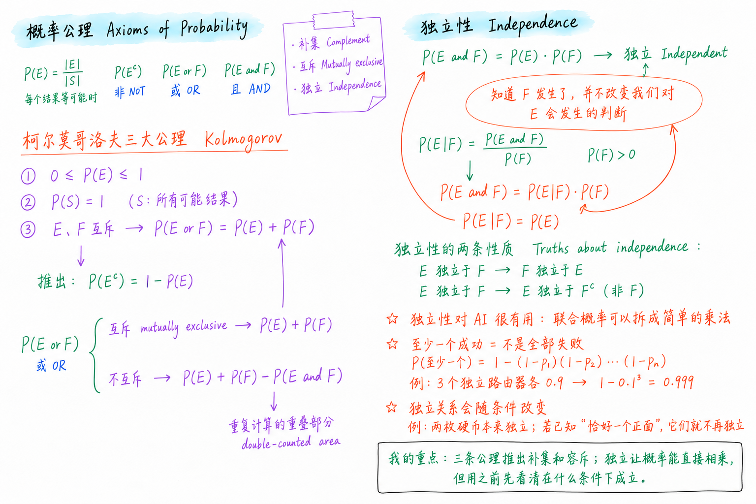
根据我的手写笔记整理,修正了三大公理的写法,并补充了简短的例子。
The big picture: from three axioms to independence
Start at the top left with the notation row: the probability of an event, and the three words NOT, OR and AND in blue. Below are Kolmogorov's three axioms in purple and the OR rule with its two branches. The sticky note at the top names the three ideas to keep: complement, mutually exclusive and independence. The right half is independence: the product rule, the circled meaning in red, conditional probability and the chain rule, and the red loop showing that the two definitions say the same thing. The red stars at the bottom right are the three points I starred in class, and my takeaway is in the corner.
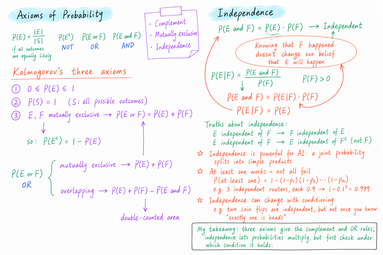
Tidied up from my handwritten page, with the axioms corrected and short examples added.
先认符号:概率常见符号和读法
概率公式很短,但每个符号都有确切的含义。能把公式正确地读出来,是理解它的第一步。下面的例子都用“掷一次均匀的六面骰子”,E =“掷出偶数”= {2, 4, 6},F =“大于 3”= {4, 5, 6}。
事件与概率
| 符号 | 读法 | 意思 | 例子(掷一次骰子) |
|---|---|---|---|
| S(也写 Ω) | 样本空间;英文读 “S”,Ω 读 “omega” | 所有可能结果组成的集合 | S = {1, 2, 3, 4, 5, 6} |
| E、F | 事件 E、事件 F;“event E” | 事件:S 的一个子集 | E = {2, 4, 6} |
| P(E) | E 的概率;“P of E”“the probability of E” | 0 到 1 之间的一个数 | P(E) = 3/6 = 0.5 |
| |E| | E 的大小(元素个数);“the size of E” | E 里有几个结果 | |E| = 3 |
| Eᶜ(也写 Ē、E′、¬E) | E 的补集、非 E;“E complement”“not E” | E 没有发生 | Eᶜ = {1, 3, 5} |
| E ∪ F | E 并 F、E 或 F;“E union F”“E or F” | 至少有一个发生 | E ∪ F = {2, 4, 5, 6} |
| E ∩ F、EF | E 交 F、E 且 F;“E intersection F”“E and F” | 两个都发生 | E ∩ F = {4, 6} |
| P(E, F) | E 和 F 的联合概率;“the joint probability of E and F” | 和 P(E ∩ F) 相同:逗号就是“且” | P(E, F) = 2/6 |
| P(E | F) | 在 F 发生的条件下 E 的概率;“the probability of E given F” | 已知 F 发生后 E 的概率。竖线读 “given”,不是除号 | P(E | F) = 2/3 |
| Fᵢ、P(Fᵢ) | F 下标 i、Fᵢ 的概率;“F sub i”“the probability of F sub i” | 一列事件 F₁、F₂、…… 中的第 i 个 | F₁ =“掷出 1” |
| P(E | Fᵢ) | 给定 Fᵢ 时 E 的概率;“the probability of E given F sub i” | 已知 Fᵢ 发生后 E 的概率 | P(偶数 | 掷出 2) = 1 |
| ∅ | 空集;“the empty set” | 没有任何结果:不可能事件 | E ∩ Eᶜ = ∅ |
| ⊆ | 是……的子集;“is a subset of” | 前者的每个结果都在后者里 | {4, 6} ⊆ E,所以 P({4, 6}) ≤ P(E) |
| E ⊥ F | E 与 F 独立;“E is independent of F” | P(E ∩ F) = P(E) · P(F) | 分开掷的两次骰子 |
| E ⊥ F | G | 在 G 的条件下 E 与 F 条件独立;“conditionally independent given G” | 已知 G 之后才独立 | 见最后一节 |
常见数学符号
| 符号 | 英文读法 | 中文 | 例子 |
|---|---|---|---|
| = | “equals”“is equal to” | 等于 | P(S) = 1 |
| ≠ | “is not equal to” | 不等于 | P(E | F) ≠ P(E) |
| > / < | “is greater than” / “is less than” | 大于 / 小于 | P(E | F) > P(E) |
| ≥ / ≤ | “is greater than or equal to” / “is less than or equal to” | 大于等于 / 小于等于 | 0 ≤ P(E) ≤ 1 |
| ≈ | “is approximately equal to” | 约等于 | 1/3 ≈ 0.33 |
| ∈ | “is an element of”“belongs to”“is in” | 属于 | 2 ∈ E |
| ∀ | “for all” | 对所有 | ∀ E:P(E) ≥ 0 |
| ∃ | “there exists” | 存在 | ∃ 一个结果属于 E ∩ F |
| ∼ | “follows”“is distributed as”(统计语境) | 服从(某个分布) | X ∼ Bernoulli(0.5) |
| Σ | “the sum of”“summation”;字母读 “sigma” | 求和 | S 中所有结果的概率之和 = 1 |
| ∏ | “the product of”;字母读 “pi” | 连乘 | 1 − ∏ (1 − pᵢ) |
| n! | “n factorial” | n 的阶乘 | 3! = 3 × 2 × 1 = 6 |
| (n k),也写 C(n, k) | “n choose k” | 从 n 个里选 k 个的组合数 | (5 选 2) = 10 |
上下标与希腊字母
这些在统计学和机器学习课程里非常常见。
| 符号 | 英文读法 | 通常表示 |
|---|---|---|
| Xᵢ | “X sub i” | 第 i 个 |
| Xᵢⱼ | “X sub i j” | 第 i 行第 j 列 |
| X² / X³ | “X squared” / “X cubed” | 平方 / 立方 |
| Xⁿ | “X to the power of n”“X to the n” | n 次方 |
| X̄ | “X bar” | X 的样本均值 |
| β̂ | “beta hat” | 由数据估计出的 β |
| μ | “mu” | 均值 |
| σ / σ² | “sigma” / “sigma squared” | 标准差 / 方差 |
| θ | “theta” | 模型参数 |
同一个横线含义不同:加在事件上,Ē 是补集(非 E);加在变量上,X̄ 是均值。两种都读 “bar”,要靠上下文区分。
完整的公式怎么读
“或”规则(容斥原理)
P(E ∪ F) = P(E) + P(F) − P(E ∩ F)
“The probability of E union F equals the probability of E plus the probability of F minus the probability of E intersection F.”
条件概率
P(E | F) = P(E ∩ F) / P(F)
“The probability of E given F equals the probability of E intersection F divided by the probability of F.” 这里的 given 是统计学里特别常用的词。
贝叶斯定理(课程后面会学)
P(Fᵢ | E) = P(E | Fᵢ) P(Fᵢ) / P(E)
“The probability of F sub i given E equals the probability of E given F sub i times the probability of F sub i, divided by the probability of E.”
全概率公式(课程后面会学;F₁ … Fₙ 要把 S 分成互不重叠的几块)
P(E) = Σᵢ₌₁ⁿ P(E | Fᵢ) P(Fᵢ)
“The probability of E equals the sum, from i equals one to n, of the probability of E given F sub i times the probability of F sub i.”
一个实用的区别:在课堂上朗读公式时,通常用简洁的说法,比如 “F sub i”“X bar”“beta hat”;解释公式含义时,则更倾向于说完整的 “the probability of event F sub i” 或 “the estimated coefficient beta”。另外两个习惯也很有用:每次看到竖线都读成 “given”(在……条件下);把“且、或、非”分别当作交集、并集和补集。不同教材常用两三种写法表达同一件事(E ∩ F、EF、P(E, F)),认得这些变体,比只背一种写法更重要。
Notation first: probability symbols and how to read them
Probability formulas are short, but each symbol carries a precise meaning. Being able to read a formula aloud is the first step to understanding it. The examples below use one roll of a fair six-sided die, with E = "an even number" = {2, 4, 6} and F = "more than 3" = {4, 5, 6}.
Events and probabilities
| Symbol | Read aloud | Meaning | Example (one die roll) |
|---|---|---|---|
| S (also Ω) | "S", the sample space; Ω is "omega" | The set of all possible outcomes | S = {1, 2, 3, 4, 5, 6} |
| E, F | "event E", "event F" | An event: a subset of S | E = {2, 4, 6} |
| P(E) | "P of E", "the probability of E" | A number from 0 to 1 | P(E) = 3/6 = 0.5 |
| |E| | "the size of E" | How many outcomes are in E | |E| = 3 |
| Eᶜ (also Ē, E′, ¬E) | "E complement", "not E" | E does not happen | Eᶜ = {1, 3, 5} |
| E ∪ F | "E union F", "E or F" | At least one of them happens | E ∪ F = {2, 4, 5, 6} |
| E ∩ F, EF | "E intersection F", "E and F" | Both happen | E ∩ F = {4, 6} |
| P(E, F) | "the joint probability of E and F" | The same as P(E ∩ F): the comma means "and" | P(E, F) = 2/6 |
| P(E | F) | "the probability of E given F" | The probability of E once we know F happened. The bar is "given", not division | P(E | F) = 2/3 |
| Fᵢ, P(Fᵢ) | "F sub i", "the probability of F sub i" | Event number i in a list F₁, F₂, … | F₁ = "roll a 1" |
| P(E | Fᵢ) | "the probability of E given F sub i" | The probability of E once we know Fᵢ happened | P(even | roll a 2) = 1 |
| ∅ | "the empty set" | No outcomes: an impossible event | E ∩ Eᶜ = ∅ |
| ⊆ | "is a subset of" | Every outcome of the first is in the second | {4, 6} ⊆ E, so P({4, 6}) ≤ P(E) |
| E ⊥ F | "E is independent of F" | P(E ∩ F) = P(E) · P(F) | two separate dice rolls |
| E ⊥ F | G | "E and F are conditionally independent given G" | Independent once G is known | see the last section |
Common math symbols
| Symbol | Read aloud | Example |
|---|---|---|
| = | "equals", "is equal to" | P(S) = 1 |
| ≠ | "is not equal to" | P(E | F) ≠ P(E) |
| > / < | "is greater than" / "is less than" | P(E | F) > P(E) |
| ≥ / ≤ | "is greater than or equal to" / "is less than or equal to" | 0 ≤ P(E) ≤ 1 |
| ≈ | "is approximately equal to" | 1/3 ≈ 0.33 |
| ∈ | "is an element of", "belongs to", "is in" | 2 ∈ E |
| ∀ | "for all" | ∀ E: P(E) ≥ 0 |
| ∃ | "there exists" | ∃ an outcome in E ∩ F |
| ∼ | "follows", "is distributed as" (statistics) | X ∼ Bernoulli(0.5) |
| Σ | "the sum of", "summation"; the letter is "sigma" | Σ P(outcome) over S = 1 |
| ∏ | "the product of"; the letter is "pi" | 1 − ∏ (1 − pᵢ) |
| n! | "n factorial" | 3! = 3 × 2 × 1 = 6 |
| (n k), also C(n, k) | "n choose k" | (5 choose 2) = 10 |
Subscripts, superscripts and Greek letters
These come up constantly in statistics and machine learning courses.
| Symbol | Read aloud | Usually means |
|---|---|---|
| Xᵢ | "X sub i" | Item number i |
| Xᵢⱼ | "X sub i j" | Row i, column j |
| X² / X³ | "X squared" / "X cubed" | Powers |
| Xⁿ | "X to the power of n", "X to the n" | Power n |
| X̄ | "X bar" | The sample mean of X |
| β̂ | "beta hat" | An estimate of β from data |
| μ | "mu" | A mean |
| σ / σ² | "sigma" / "sigma squared" | Standard deviation / variance |
| θ | "theta" | A model parameter |
The same bar means different things: over an event, Ē is the complement ("not E"); over a variable, X̄ is the mean. Read it as "bar" in both cases and tell them apart from context.
Reading a whole formula aloud
The OR rule (inclusion–exclusion)
P(E ∪ F) = P(E) + P(F) − P(E ∩ F)
"The probability of E union F equals the probability of E plus the probability of F minus the probability of E intersection F."
Conditional probability
P(E | F) = P(E ∩ F) / P(F)
"The probability of E given F equals the probability of E intersection F divided by the probability of F."
Bayes' theorem (later in the course)
P(Fᵢ | E) = P(E | Fᵢ) P(Fᵢ) / P(E)
"The probability of F sub i given E equals the probability of E given F sub i times the probability of F sub i, divided by the probability of E."
The law of total probability (later in the course; F₁ … Fₙ must split S into non-overlapping pieces)
P(E) = Σᵢ₌₁ⁿ P(E | Fᵢ) P(Fᵢ)
"The probability of E equals the sum, from i equals one to n, of the probability of E given F sub i times the probability of F sub i."
A practical difference: when reading a formula aloud in class, people use the short forms, such as "F sub i", "X bar" and "beta hat". When explaining what it means, they use fuller phrases, such as "the probability of event F sub i" or "the estimated coefficient beta". Two more habits help: read the vertical bar as "given" every time, and read "and", "or" and "not" as set operations (intersection, union and complement). Textbooks often write one idea in two or three ways (E ∩ F, EF, P(E, F)), so recognising the variants matters more than memorising one.
看视频这一段 / Watch this part 看专题视频 / Watch the special video: 概率符号英文怎么读
柯尔莫哥洛夫三大公理
现代概率论建立在数学家柯尔莫哥洛夫(Andrey Kolmogorov)1933 年提出的三条公理之上。公理是不需要证明、直接接受的规则,其他规则都由它们推出来。
| 公理 | 符号 | 意思 |
|---|---|---|
| 1 | 0 ≤ P(E) ≤ 1 | 任何概率都在 0 到 1 之间 |
| 2 | P(S) = 1 | 样本空间里总有某个结果会发生 |
| 3 | 若 E ∩ F = ∅,则 P(E or F) = P(E) + P(F) | 互斥事件的概率可以直接相加 |
当每个结果等可能时,概率就是计数:P(E) = |E| / |S|。掷出偶数的概率是 3/6。这个计数公式只是特例,不是定义:一颗灌了铅的骰子仍然满足三条公理,却不满足 |E| / |S|。
我的手写笔记把 P(E) + P(Eᶜ) = 1 写在“柯尔莫哥洛夫三大公理”旁边。这个等式是对的,但它不是公理之一,而是由公理推出的第一条规则(见下一节)。被它替换掉的那条公理是 P(S) = 1。
Kolmogorov's three axioms
Modern probability rests on three axioms set out by the mathematician Andrey Kolmogorov in 1933. An axiom is a rule accepted without proof; everything else is derived from it.
| Axiom | In symbols | In words |
|---|---|---|
| 1 | 0 ≤ P(E) ≤ 1 | Every probability is between 0 and 1 |
| 2 | P(S) = 1 | Something in the sample space always happens |
| 3 | If E ∩ F = ∅, then P(E or F) = P(E) + P(F) | For mutually exclusive events, probabilities add |
When every outcome is equally likely, a probability is a count: P(E) = |E| / |S|. For an even number on a die that is 3/6. This counting formula is a special case, not a definition: a loaded die still obeys the three axioms, but not |E| / |S|.
My handwritten page wrote P(E) + P(Eᶜ) = 1 next to "Kolmogorov's three axioms". That equation is true, but it is not one of the axioms; it is the first rule derived from them (next section). The axiom it replaced is P(S) = 1.
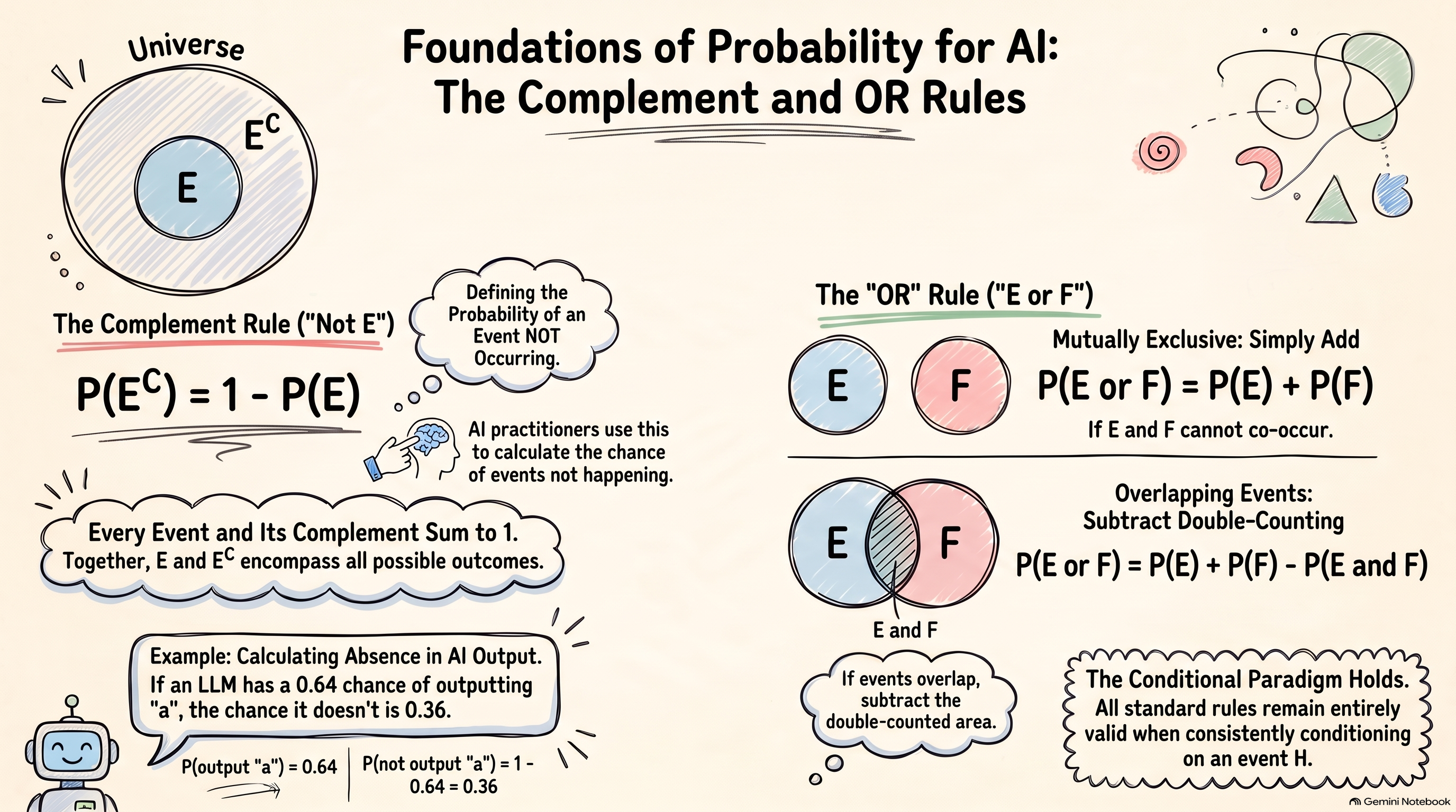
非:补集规则
E 和 Eᶜ 互斥,合起来正好是整个样本空间。由公理 2 和公理 3 得到 P(E) + P(Eᶜ) = P(S) = 1,所以
P(Eᶜ) = 1 − P(E)
当“E 不发生”比“E 发生”更容易计算时,这条规则最有用。如果语言模型给下一个词是 “a” 的概率为 0.64,那么下一个词是其他任何词的概率就是 1 − 0.64 = 0.36。
NOT: the complement rule
E and Eᶜ are mutually exclusive, and together they make up the whole sample space. Axioms 2 and 3 therefore give P(E) + P(Eᶜ) = P(S) = 1, so
P(Eᶜ) = 1 − P(E)
This rule is most useful when "not E" is easier to count than E. If a language model gives the word "a" a 0.64 chance of being next, the chance that the next word is anything else is 1 − 0.64 = 0.36.
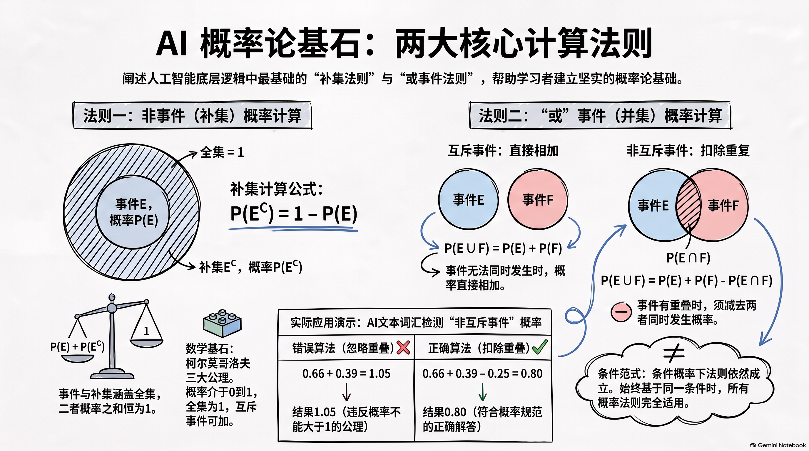
或:相加时别重复计算
P(E or F) 怎么算,取决于两个事件能不能同时发生。
| 情况 | 规则 | 骰子例子(E = 偶数,F = 大于 3) |
|---|---|---|
| 互斥:E ∩ F = ∅ | P(E or F) = P(E) + P(F) | E = {2},F = {5}:1/6 + 1/6 = 2/6 |
| 不互斥(有重叠) | P(E or F) = P(E) + P(F) − P(E and F) | 3/6 + 3/6 − 2/6 = 4/6 |
第二行叫容斥原理(inclusion–exclusion)。把 P(E) 和 P(F) 相加时,两者共有的结果(这里是 4 和 6)被算了两次,所以要减去一次重叠部分。如果忘了减,算出来的“概率”可能超过 1,这时很容易发现。
OR: adding probabilities without double counting
P(E or F) depends on whether the two events can happen together.
| Case | Rule | Die example (E = even, F = more than 3) |
|---|---|---|
| Mutually exclusive: E ∩ F = ∅ | P(E or F) = P(E) + P(F) | E = {2}, F = {5}: 1/6 + 1/6 = 2/6 |
| Overlapping | P(E or F) = P(E) + P(F) − P(E and F) | 3/6 + 3/6 − 2/6 = 4/6 |
The second line is called inclusion–exclusion. Adding P(E) and P(F) counts the outcomes in both, here 4 and 6, twice, so the overlap is subtracted once. Forgetting it is easy to spot when the "probability" comes out above 1.
条件概率与链式法则
在 F 发生的条件下 E 的概率,就是已知 F 已经发生后,E 发生的概率:
P(E | F) = P(E and F) / P(F),要求 P(F) > 0。
知道 F 发生,相当于把可能的结果缩小到 F 里面,再问其中有多大比例也属于 E。掷骰子时,已知点数大于 3,只剩 {4, 5, 6},其中两个是偶数,所以 P(偶数 | 大于 3) = 2/3,比原来的 1/2 高。
两边同乘 P(F),就得到链式法则:
P(E and F) = P(E | F) · P(F)
上面所有规则在同一个条件下也都成立,比如 P(Eᶜ | G) = 1 − P(E | G),只要每一项都以同一个 G 为条件。
Conditional probability and the chain rule
The conditional probability of E given F is the probability of E once we know F has happened:
P(E | F) = P(E and F) / P(F), defined when P(F) > 0.
Knowing F shrinks the world to the outcomes in F, and we ask what share of them are also in E. On the die, knowing the roll is more than 3 leaves {4, 5, 6}; two of those are even, so P(even | more than 3) = 2/3, up from 1/2.
Multiplying both sides by P(F) gives the chain rule:
P(E and F) = P(E | F) · P(F)
All the rules above also hold inside a condition: P(Eᶜ | G) = 1 − P(E | G), for example, as long as every term is conditioned on the same G.
独立性
如果知道 F 发生了,并不改变我们对 E 会发生的判断,E 和 F 就是独立的:
P(E | F) = P(E)
把它代入链式法则,就得到乘法规则:P(E and F) = P(E) · P(F)。两种写法说的是同一件事,全景图里的红色回环画的就是这一步。分开掷的两次骰子是独立的:第一次的点数对第二次毫无影响,所以 P(两次都是 6) = 1/6 × 1/6 = 1/36。
由定义可以推出独立性的两条性质:
- 对称:E 独立于 F,则 F 也独立于 E。
- 对补集也成立:E 独立于 F,则 E 也独立于 Fᶜ(非 F)。知道 F 没有发生,同样不提供关于 E 的信息。
独立不等于互斥。互斥事件不能同时发生,知道其中一个发生了,就知道另一个没有发生:这恰恰是很强的相关。
独立性对 AI 很有用,因为它能把一个难算的联合概率拆成几个简单概率的乘积。没有独立性,模型要估计很多事情一起出现的概率;有了独立性,每一部分可以单独估计,再相乘。
Independence
E and F are independent when knowing that F happened does not change our belief that E will happen:
P(E | F) = P(E)
Put that into the chain rule and the product rule appears: P(E and F) = P(E) · P(F). The two forms say the same thing; the red loop in the big picture shows that step. Two separate rolls of a die are independent: the first roll tells you nothing about the second, so P(two sixes) = 1/6 × 1/6 = 1/36.
Two truths about independence follow from the definition:
- It is symmetric: if E is independent of F, then F is independent of E.
- It carries over to complements: if E is independent of F, then E is also independent of Fᶜ. Knowing that F did not happen tells you just as little.
Independent is not the same as mutually exclusive. Mutually exclusive events cannot happen together, so learning that one happened tells you the other did not: that is strong dependence.
Independence is powerful for AI because it turns one hard joint probability into a product of simple ones. Without it, a model has to estimate how many things behave together; with it, each piece can be estimated on its own and multiplied.
至少一个成功 = 不是全部失败
“至少一个”的问题直接相加很难算,用补集就容易了。如果 n 个部件各自独立地以概率 p₁ … pₙ 正常工作:
P(至少一个成功) = 1 − P(全部失败) = 1 − (1 − p₁)(1 − p₂)…(1 − pₙ)
补集把“或”变成“且”,独立性再把“且”变成乘法。课程讲义里的例子:三个独立的路由器各有 0.9 的概率正常工作,至少有一条通路可用的概率是 1 − 0.1³ = 0.999。
At least one works = not all fail
"At least one" questions are hard to add up directly, but easy through the complement. If n parts work independently with probabilities p₁ … pₙ:
P(at least one works) = 1 − P(all fail) = 1 − (1 − p₁)(1 − p₂)…(1 − pₙ)
The complement turns OR into AND, and independence turns AND into multiplication. In the course reader's example, three independent routers that each work with probability 0.9 give a working path with probability 1 − 0.1³ = 0.999.
独立关系会随条件改变
两个事件是否独立,在加入第三个事件作为条件后可能会改变。
- 独立可以变成不独立。 两枚均匀硬币的结果本来相互独立。现在假设我们知道恰好有一枚是正面:如果第一枚是正面,第二枚就一定是反面。在这个信息下,它们不再独立。
- 不独立可以变成独立。 同一家诊所两位患者的化验结果,可能因为送到同一个实验室而一起偏高或偏低;一旦知道是哪家实验室做的检测,两人的结果就可以相互独立。
这叫条件独立,写作 E ⊥ F | G。在 G 的条件下独立,不代表去掉 G 之后也独立,反过来也不成立。所以每次计算时,都值得确认它假设的是哪个条件。
Independence can change with conditioning
Whether two events are independent can change once we condition on a third event.
- Independent can become dependent. Two fair coin flips are independent. Now suppose we learn that exactly one of them landed heads. If the first flip was heads, the second must be tails: given that information, they are no longer independent.
- Dependent can become independent. The test results of two patients from the same clinic may move together because they share the same lab; once we know which lab ran the tests, the results can be independent of each other.
This is called conditional independence, written E ⊥ F | G. Being conditionally independent given G does not mean being independent without G, and the reverse is not true either, so it is worth checking each time which condition a calculation assumes.
我的思考
第一节课的体验是,如果能早点接触到这样的上课方式,我肯定会更喜欢数学。Chris Piech 的课讲得简单易懂。我的总结整理了所有重要的概念,但如果想进一步理解,真的很推荐上这门课。
在学概念之前,我先补充学习了概率相关符号的表达,因为能把公式正确地读出来,就理解了一半。之后需要知道的概念并不多。柯尔莫哥洛夫三大公理:事件的概率在 0 到 1 之间;整个样本空间的概率为 1;如果 E 和 F 没有交集,那么 E 或 F 发生的概率是两件事单独发生的概率之和。“事件发生和不发生的概率相加为 1”这条补集规则,就是由它们推出来的。如果 E 和 F 不互斥,概率之和还要减去计算了两遍的部分,也就是 E 和 F 同时发生的概率。
什么是独立事件?事件 F 的发生并不影响事件 E 的发生。这时两者同时发生的概率是 P(E) × P(F),条件概率 P(E | F) = P(E and F) / P(F) 解释了为什么。E 独立于 F,则 F 独立于 E;E 独立于 F,则 E 也独立于非 F。我标星的两点:“至少一个成功”就是“不是全部失败”;独立关系会随条件改变。
My thoughts
My experience of the first lesson: if I had been taught this way earlier, I would certainly have liked mathematics more. Chris Piech's teaching is simple and easy to follow. This note collects the important concepts, but if you want to understand them more deeply, I really recommend taking the course.
Before the concepts I studied the symbols, because reading a formula aloud correctly is half of understanding it. After that, the concepts to know are few. Kolmogorov's three axioms: every probability is between 0 and 1, the whole sample space has probability 1, and if E and F do not overlap, the probability of E or F is the sum of their probabilities. The complement rule, that an event happening and not happening add up to 1, follows from them. If E and F do overlap, the sum has to subtract the part counted twice, the probability that E and F both happen.
Independence means that F happening does not affect whether E happens; then the probability of both is P(E) × P(F), and conditional probability, P(E | F) = P(E and F) / P(F), shows why. If E is independent of F, then F is independent of E, and E is also independent of not F. Two points I starred: "at least one works" is the same as "not all fail", and an independence relationship can change with conditioning.
原始手写笔记
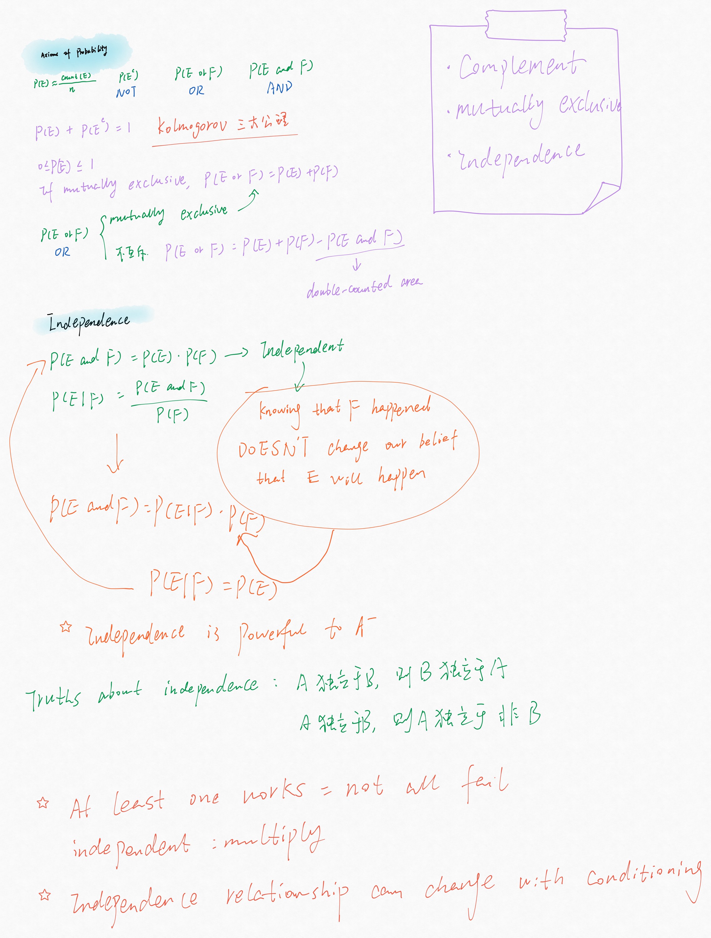
整理后的版本改了这些地方:“Axiome”改为 Axioms;P(E) = count(E)/n 写成 P(E) = |E| / |S|,并注明只在每个结果等可能时成立;柯尔莫哥洛夫三大公理改为 0 ≤ P(E) ≤ 1、P(S) = 1 和互斥事件的加法规则,P(Eᶜ) = 1 − P(E) 标为由公理推出、而不是公理本身;P(E | F) 补上了条件 P(F) > 0;红色回环注明是在说明两种独立性定义等价;“independent: multiply”写成公式 1 − (1 − p₁)…(1 − pₙ),并加了三个路由器的例子;“Independence is powerful to AI”补了一句原因;“独立关系会随条件改变”加了两枚硬币的例子。
Original handwritten notes
What changed in the tidied version: "Axiome" is now Axioms; P(E) = count(E)/n is written P(E) = |E| / |S| and marked as holding only when every outcome is equally likely; Kolmogorov's three axioms are now listed as 0 ≤ P(E) ≤ 1, P(S) = 1 and the addition rule for mutually exclusive events, with P(Eᶜ) = 1 − P(E) shown as derived from them rather than as an axiom; P(E | F) gained the condition P(F) > 0; the red loop is labelled as showing the two definitions of independence are equivalent; "independent: multiply" became the formula 1 − (1 − p₁)…(1 − pₙ) with the three-router example; "Independence is powerful to AI" gained a short reason; "independence can change with conditioning" gained the two-coin example.
学习来源与资源
这篇笔记基于我在斯坦福免费在线课程 Probability for AI(PAI,由 Chris Piech 和 Mehran Sahami 主讲)第一周的学习笔记。定义和例子已对照课程讲义核对:
- Chris Piech,Probability for Computer Scientists(CS109 课程讲义):Axioms of Probability、Conditional Probability 和 Independence(含路由器网络的例子)。
- A. N. Kolmogorov(1933),Grundbegriffe der Wahrscheinlichkeitsrechnung;英译本 Foundations of the Theory of Probability(1950)。
自己动手试试
- Seeing Theory: Basic Probability(布朗大学,英文):交互式的抛硬币、掷骰子模拟,看试验次数增加时概率怎样稳定下来。
- Seeing Theory: Compound Probability:拖动维恩图,观察并集、交集和条件概率的变化。
Learning sources and resources
This note is based on my study notes from week 1 of Probability for AI (PAI), Stanford's free online course taught by Chris Piech and Mehran Sahami. Definitions and examples were checked against the course's reader:
- Chris Piech, Probability for Computer Scientists, the CS109 course reader: Axioms of Probability, Conditional Probability and Independence (including the router network example).
- A. N. Kolmogorov (1933), Grundbegriffe der Wahrscheinlichkeitsrechnung; English translation Foundations of the Theory of Probability (1950).
Try it yourself
- Seeing Theory: Basic Probability (Brown University): interactive coin and die simulations that show probabilities settling as the number of trials grows.
- Seeing Theory: Compound Probability: drag Venn diagrams to see unions, intersections and conditional probability change.