从顶部的标题开始，先读左半边：随机变量的定义，PMF 和它的柱状图，一条绿色箭头连到“AI 的下一个词”，下面是期望和方差，都用掷骰子做例子。右半边从上往下是伯努利 → 二项 → 泊松，蓝色下划线标出“n 很大、p 很小”这个条件，红色是泊松近似的经验法则，绿色是泊松在空间和时间建模上的拓展。底部紫色的一行是水印：怎样通过改变概率影响 AI 生成的内容。右下角是我的总结。

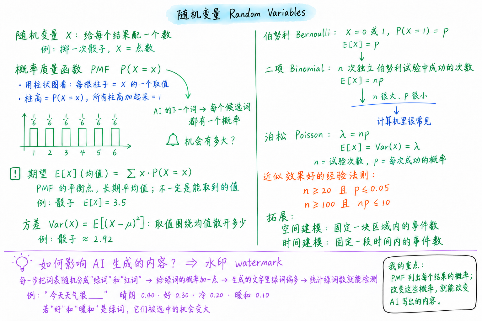
✎ 阅读提示根据我的手写笔记整理，做了几处修正和补充。

Start with the title at the top, then read the left half: the definition of a random variable, the PMF and its bar chart with a green arrow to "AI's next word", then expectation and variance, each with a die example. The right half runs down the chain Bernoulli → binomial → Poisson; the blue underline marks the condition "n large, p small", the red lines are the rule of thumb for the Poisson approximation, and the green lines extend Poisson to modelling space and time. The purple line along the bottom is the watermark: how changing probabilities steers what an AI generates. My takeaway is in the bottom-right corner.

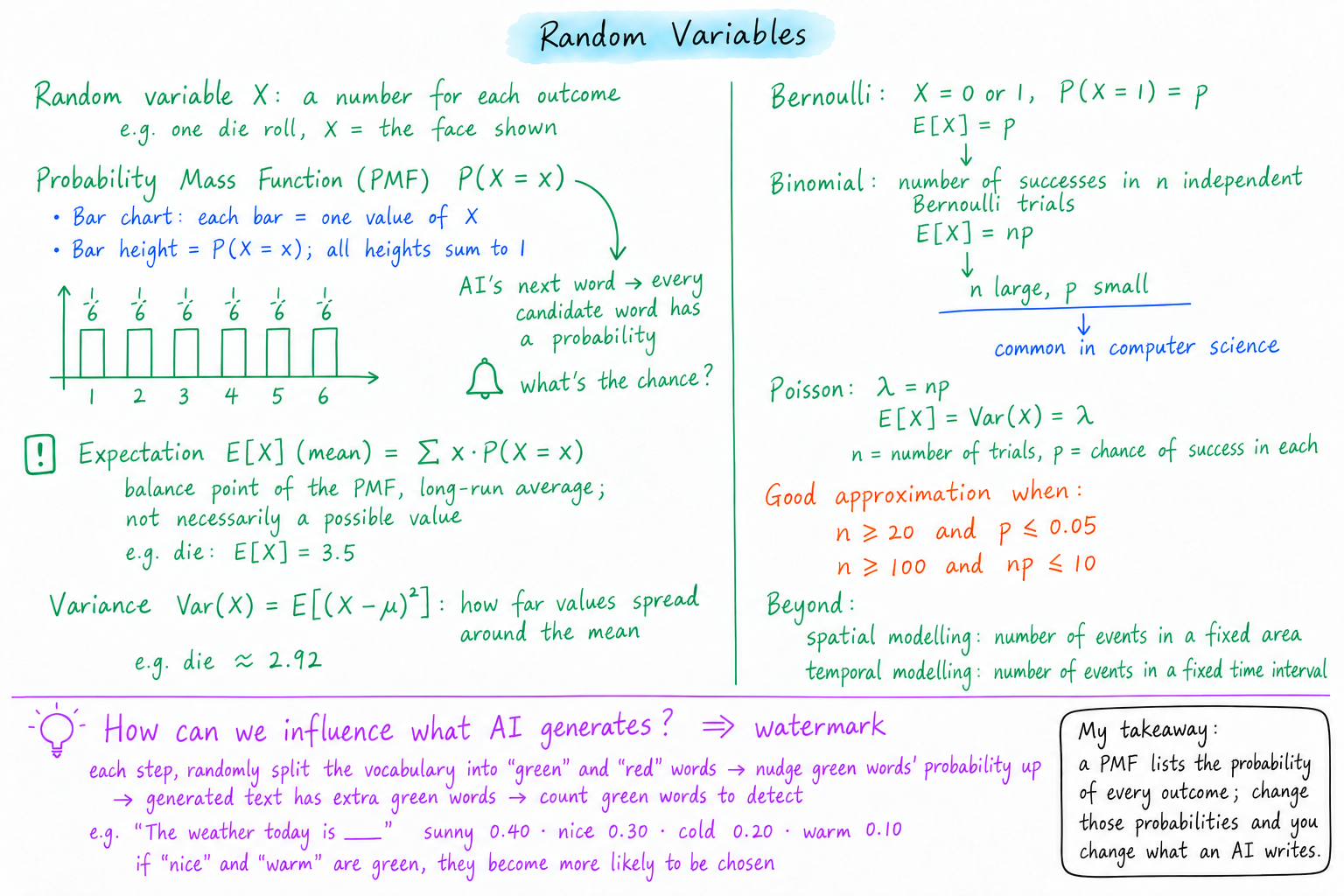
✎ 阅读提示Tidied up from my handwritten page, with a few corrections and additions.

随机变量（random variable）通常记作大写的 X，它给随机试验的每个结果配一个数。掷一次骰子，X 就是朝上的点数，可能取 1 到 6；抛 10 次硬币，X 可以是正面出现的次数，可能取 0 到 10。

有了数，就能做计算：求平均、比大小、算分散程度。上一周的事件（比如“掷出偶数”）在这里可以写成 X 的取值：P(X ∈ {2, 4, 6}) = 0.5。小写的 x 表示 X 可能取到的某个具体值。

A random variable, usually written as a capital X, assigns a number to each outcome of a random experiment. For one die roll, X is the face that comes up, from 1 to 6; for ten coin flips, X can be the number of heads, from 0 to 10.

Once outcomes are numbers we can calculate with them: average them, compare them, measure how spread out they are. Last week's events, such as "roll an even number", can now be written as values of X: P(X ∈ {2, 4, 6}) = 0.5. A lower-case x stands for one particular value that X can take.

概率质量函数（probability mass function，PMF）列出离散随机变量每个可能取值的概率，写作 P(X = x)。它最常画成柱状图：

看柱状图的什么	含义	掷一枚公平的骰子
横轴上的每根柱子	X 的一个可能取值 x	1、2、3、4、5、6
柱子的高度	P(X = x)	每根都是 1/6
所有柱高之和	必须等于 1	6 × 1/6 = 1

如果手上只有数据，把每个取值出现的次数除以总次数，得到的“归一化直方图”就是 PMF 的近似。

在 AI 里，大语言模型每生成一个词，都会对词表里的每个候选词给出一个概率，这就是一个 PMF：柱子是词，柱高是“下一个词是它”的概率，加起来等于 1。模型再按这个分布抽出一个词。

The probability mass function (PMF) lists the probability of every possible value of a discrete random variable, written P(X = x). It is usually drawn as a bar chart:

In the bar chart	Meaning	One fair die
Each bar on the horizontal axis	One possible value x of X	1, 2, 3, 4, 5, 6
The height of a bar	P(X = x)	1/6 for every bar
All bar heights together	Must add up to 1	6 × 1/6 = 1

With data instead of a model, divide the count of each value by the total number of observations: this normalised histogram approximates the PMF.

In AI, every time a large language model generates a word it gives each candidate in its vocabulary a probability. That is a PMF: the bars are words, each height is the chance that the next word is that one, and the heights add up to 1. The model then draws one word from this distribution.

期望（expectation）E[X]，也叫均值（mean），是每个取值乘以它的概率再加起来：

E[X] = Σ x · P(X = x)

把 PMF 的柱子想成放在横轴上的重物，期望就是让横轴保持平衡的那个支点；它也是试验重复很多次后的长期平均值。

掷骰子：E[X] = (1 + 2 + 3 + 4 + 5 + 6) × 1/6 = 3.5。骰子上没有 3.5，所以期望不一定是能取到的值，它描述的是“平均起来在哪里”，不是“最可能出现什么”。

The expectation E[X], also called the mean, multiplies each value by its probability and adds them up:

E[X] = Σ x · P(X = x)

Picture the bars of the PMF as weights resting on the horizontal axis: the expectation is the point where the axis balances. It is also the long-run average if the experiment is repeated many times.

For a die: E[X] = (1 + 2 + 3 + 4 + 5 + 6) × 1/6 = 3.5. No face shows 3.5, so the expectation need not be a value X can take. It tells you where the values average out, not which value is most likely.

方差（variance）衡量取值离均值有多远，μ 表示均值 E[X]：

Var(X) = E[(X − μ)²]

也可以用更好算的形式 Var(X) = E[X²] − (E[X])²。掷骰子：E[X²] = (1 + 4 + 9 + 16 + 25 + 36) / 6 ≈ 15.17，所以 Var(X) ≈ 15.17 − 3.5² ≈ 2.92。方差的平方根是标准差，单位和 X 相同，更容易直观理解。

两个分布可以期望相同、方差不同：一个总是掷出 3 或 4，另一个总是掷出 1 或 6，平均都是 3.5，后者散得开得多。

The variance measures how far the values fall from the mean, written μ = E[X]:

Var(X) = E[(X − μ)²]

The equivalent form Var(X) = E[X²] − (E[X])² is easier to compute. For a die: E[X²] = (1 + 4 + 9 + 16 + 25 + 36) / 6 ≈ 15.17, so Var(X) ≈ 15.17 − 3.5² ≈ 2.92. The square root of the variance is the standard deviation, which has the same units as X and is easier to picture.

Two distributions can share a mean and differ in variance: a die that only ever shows 3 or 4 and one that only shows 1 or 6 both average 3.5, but the second is far more spread out.

三种分布是一条链：二项由多次伯努利试验组成，泊松又是二项在特定条件下的近似。

分布	X 表示什么	参数	期望	方差	例子
伯努利 Bernoulli	一次试验成功为 1，否则为 0	p：成功的概率	p	p(1 − p)	抛一次硬币是否正面；一封邮件是不是垃圾邮件
二项 Binomial	n 次独立伯努利试验中成功的次数	n：试验次数；p：每次成功的概率	np	np(1 − p)	抛 10 次硬币，正面出现几次
泊松 Poisson	固定时间或区域内事件发生的次数	λ：平均发生次数	λ	λ	一分钟内网站收到多少次访问

伯努利只有“是”和“否”两个结果。二项把同一个伯努利试验独立地重复 n 次，数成功了几次：抛 10 次公平硬币，恰好 3 次正面的概率是 C(10, 3) / 2¹⁰ = 120 / 1024 ≈ 0.117，平均会有 10 × 0.5 = 5 次正面。

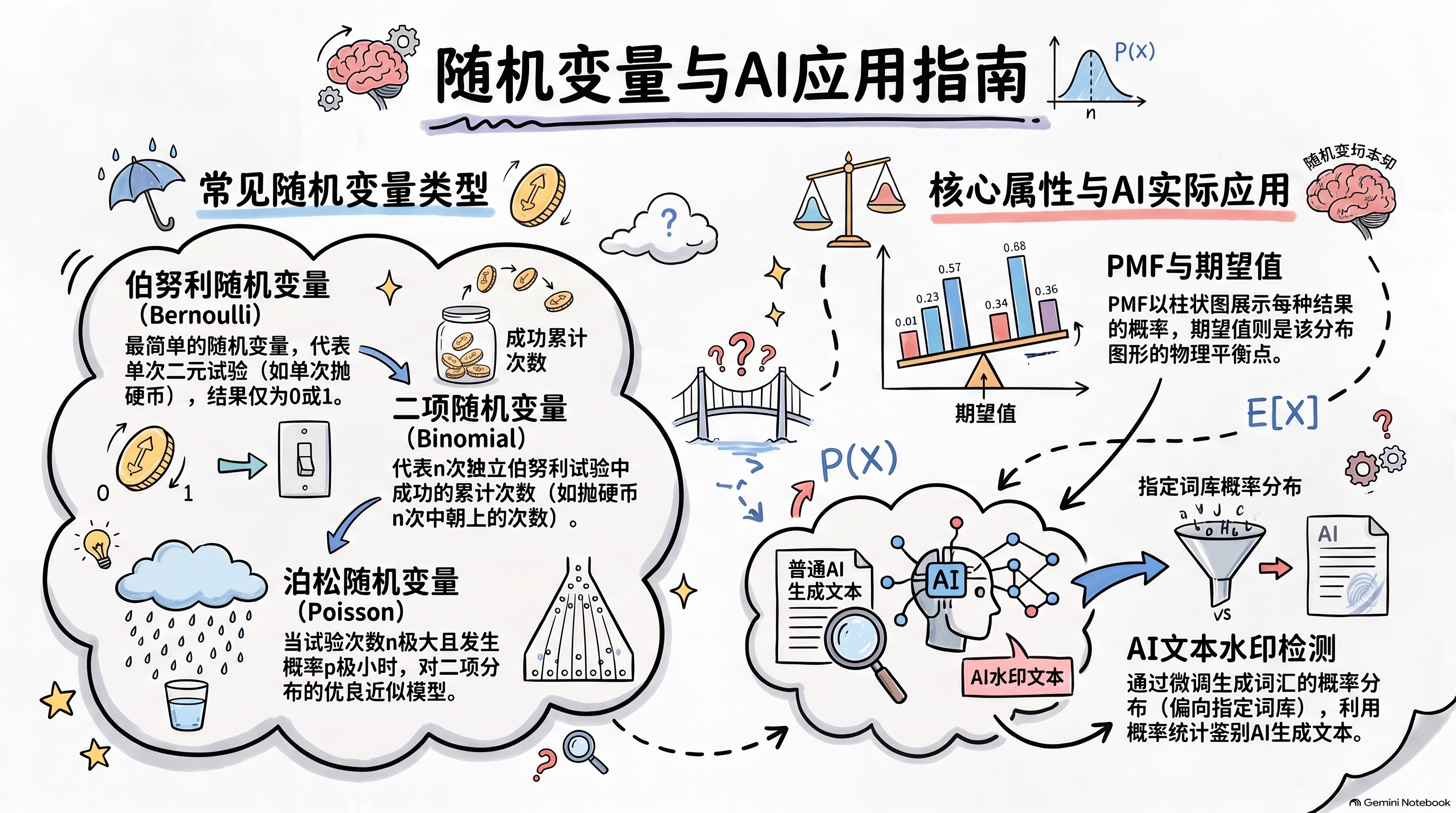
✎ 阅读提示读图提示：右上角 PMF 柱状图标的几个概率加起来超过 1，真正的 PMF 所有柱高之和必须等于 1，这里只是示意。

The three form a chain: a binomial is built from repeated Bernoulli trials, and a Poisson approximates a binomial under particular conditions.

Distribution	What X counts	Parameters	Mean	Variance	Example
Bernoulli	1 if one trial succeeds, otherwise 0	p: probability of success	p	p(1 − p)	Does one coin flip land heads? Is an email spam?
Binomial	Successes in n independent Bernoulli trials	n: number of trials; p: probability of success in each	np	np(1 − p)	Number of heads in 10 coin flips
Poisson	Events in a fixed interval of time or region of space	λ: average number of events	λ	λ	Visits to a website in one minute

Bernoulli has only two outcomes, yes or no. Binomial repeats the same Bernoulli trial n times independently and counts the successes: in 10 flips of a fair coin, the chance of exactly 3 heads is C(10, 3) / 2¹⁰ = 120 / 1024 ≈ 0.117, and on average there are 10 × 0.5 = 5 heads.

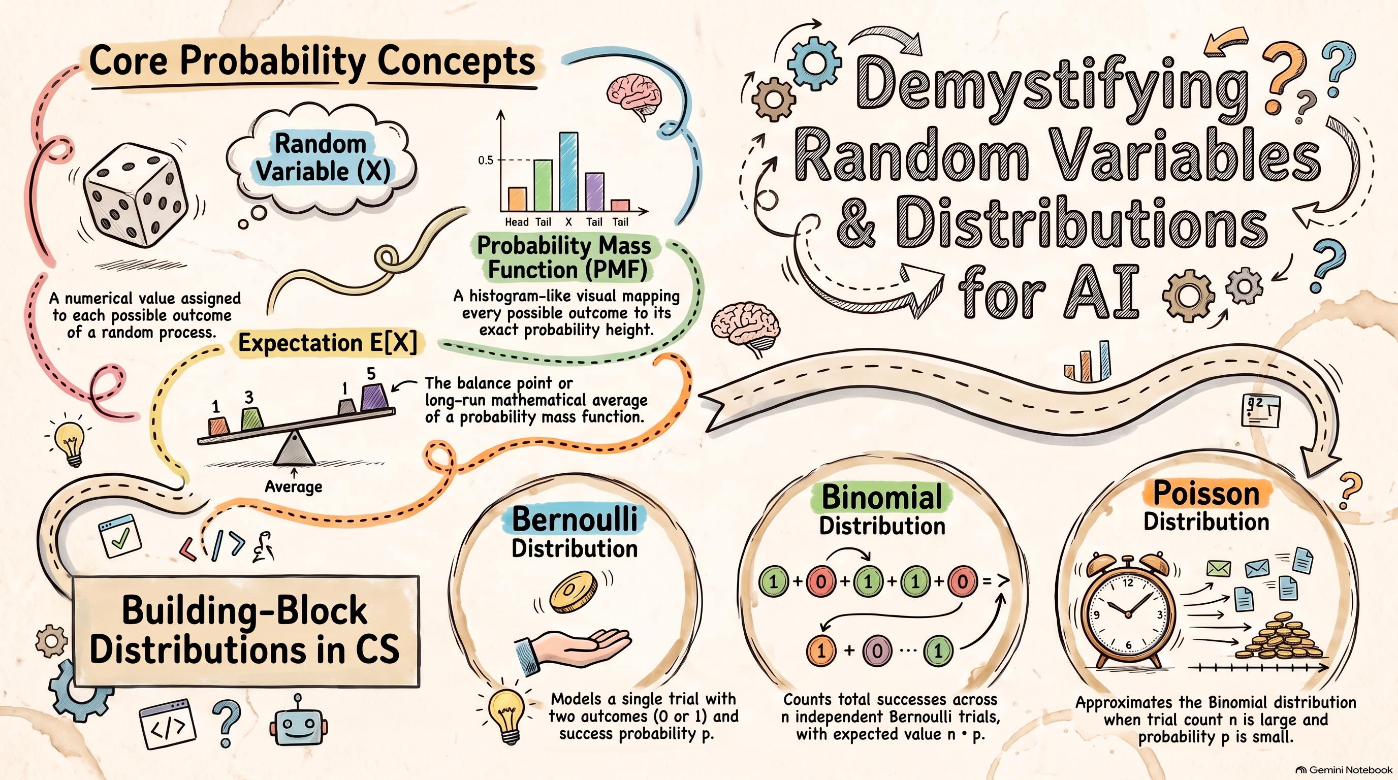
✎ 阅读提示A reading note: the labels under the PMF bar chart (Head, Tail, X, Tail, Tail) do not match any real random variable. Read it as a picture of bars and heights, as in the die table above.

当二项分布的试验次数 n 很大、每次成功的概率 p 很小时，直接算二项很麻烦，这时可以用泊松分布近似，令 λ = np：

P(X = k) = λᵏ e^(−λ) / k!

例子：一个网页一天有 1000 次访问，每次访问点开某个广告的概率是 0.002。点击次数严格来说服从二项分布（n = 1000，p = 0.002），用泊松近似时 λ = 1000 × 0.002 = 2，一次都没人点的概率是 e^(−2) ≈ 0.135，和二项的精确结果 0.998¹⁰⁰⁰ ≈ 0.135 几乎一样。n 越大，近似越准。

近似效果好的常用经验法则：

• n ≥ 20 且 p ≤ 0.05；
• n ≥ 100 且 np ≤ 10。

这种“试验很多、每次的概率很小”的情况在计算机里很常见：服务器每分钟收到的请求数、一段文本里的拼写错误数、网络里丢失的数据包数。

拓展：空间与时间建模。泊松分布不只是二项的近似，它本身就用来数“固定范围内的事件数”，前提是事件以稳定的平均速率、彼此独立地发生。

• 时间建模：固定一段时间内的事件数，例如每小时到达急诊的病人数。
• 空间建模：固定一块区域内的事件数，例如一平方公里内的病例数，或显微镜一个视野里的细胞数。

一个经典的历史例子：1898 年，拉迪斯劳斯·博特基维茨（Ladislaus Bortkiewicz）统计了普鲁士骑兵军团每年被马踢死的士兵人数，发现这些罕见事件的次数和泊松分布吻合得很好。

When a binomial has a large number of trials n and a small probability p, computing it directly is awkward, and a Poisson distribution with λ = np approximates it well:

P(X = k) = λᵏ e^(−λ) / k!

An example: a web page gets 1,000 visits a day, and each visit clicks a certain ad with probability 0.002. Strictly, the number of clicks is binomial (n = 1,000, p = 0.002). The Poisson approximation uses λ = 1,000 × 0.002 = 2, so the chance of no clicks at all is e^(−2) ≈ 0.135, almost exactly the binomial answer 0.998¹⁰⁰⁰ ≈ 0.135. The larger n is, the better the approximation.

Common rules of thumb for when the approximation works well:

• n ≥ 20 and p ≤ 0.05;
• n ≥ 100 and np ≤ 10.

"Many trials, each unlikely" is common in computer science: requests reaching a server each minute, typos in a document, packets lost on a network.

Beyond the binomial: modelling space and time. The Poisson distribution is more than an approximation. It counts events in a fixed range directly, as long as they happen independently at a steady average rate.

• Temporal modelling: the number of events in a fixed interval of time, such as patients arriving at an emergency department each hour.
• Spatial modelling: the number of events in a fixed area, such as cases per square kilometre or cells in one microscope field.

A classic piece of history: in 1898 Ladislaus Bortkiewicz counted the soldiers killed by horse kicks each year in corps of the Prussian cavalry and found that these rare events followed a Poisson distribution closely.

既然大语言模型每一步都按下一个词的 PMF 抽样，那么只要悄悄改变这个 PMF，就能影响它写出的文字。文本水印（watermark）就是这样做的。Kirchenbauer 等人（2023）的方法是：

1. 分组：生成每个词之前，用前一个词做随机种子，把整个词表随机分成“绿词”和“红词”两组（例如各一半）。
2. 加一点权重：给所有绿词的分数加上一个常数，绿词被选中的概率就变大了；红词并没有被禁止。
3. 检测：拿到一段文字后，用同样的种子重建每一步的绿词表，数一数绿词占多少。人写的文字大约一半是绿词；带水印的文字绿词明显偏多，用一个 z 检验就能判断。

一个例子。模型要补全“今天天气很___”，原来的 PMF 是：晴朗 0.40、好 0.30、冷 0.20、暖和 0.10。如果这一步“好”和“暖和”是绿词，加上权重后（论文实验里常用的强度 δ = 2）大约变成：好 0.62、暖和 0.21、晴朗 0.11、冷 0.06。四个词仍然都可能出现，只是更偏向绿词。一段 200 个词的文字，人写的大约有 100 个绿词；如果数出来有 150 个，z = (150 − 100) / √(200 × 0.25) ≈ 7.1，远高于论文用的阈值 4，基本可以判定带有水印。

需要注意：分组是随机的，和词常不常见无关；当下一个词几乎只有一个合理选择时（比如“中华人民共和___”），加权几乎改变不了结果，所以这类低多样性的文字很难加上水印。

Because a large language model samples every word from a PMF over the next word, quietly changing that PMF changes the text it produces. A text watermark does exactly this. In the method of Kirchenbauer and colleagues (2023):

1. Split: before each word is generated, the previous word seeds a random split of the whole vocabulary into a "green" list and a "red" list (for example half each).
2. Nudge: a constant is added to the score of every green word, so green words become more likely. Red words are not banned.
3. Detect: given a text, rebuild each step's green list with the same seed and count the green words. Human writing is about half green; watermarked text has clearly more, and a z-test says how unlikely that is by chance.

An example. The model is completing "The weather today is ___", and the original PMF is: sunny 0.40, nice 0.30, cold 0.20, warm 0.10. If "nice" and "warm" are green at this step, the nudge (δ = 2, a strength used in the paper's experiments) shifts it to about nice 0.62, warm 0.21, sunny 0.11, cold 0.06. All four words can still appear; the choice just leans green. In a 200-word text, a person would write about 100 green words. If we count 150, z = (150 − 100) / √(200 × 0.25) ≈ 7.1, far above the paper's threshold of 4, so the text almost certainly carries the watermark.

Two things to keep in mind: the split is random, not based on how common a word is; and when only one next word makes sense (such as "Barack ___"), the nudge barely changes anything, so text with little room for choice is hard to watermark.

这一周要了解的定义不多。概率质量函数 PMF 用柱状图展示，每根柱子是一个可能结果的概率，所有柱子加起来等于 1；放到 AI 里，就是预测一个序列里下一个词的机会有多大。期望和方差可以简单理解：期望是 PMF 的平衡点，方差是取值围绕均值散开多少。

重要的是三个分布。伯努利只有是和否两个结果；二项是同样的是/否试验重复多次，数成功了几次；泊松适用于 n 很大、p 很小的情况，现实中经常用到，还可以拓展到空间建模和时间序列建模。

我最感兴趣的是：可以通过改变概率来影响 AI 生成的内容。在一句话里很多词都可能出现，但如果把一部分词的概率调高，模型就会更多地从这些词里选，水印就是这样做出来的。课程还有一个有意思的地方：老师会讲讲发现这些分布的人。

This week has only a few definitions to learn. The probability mass function is shown as a bar chart: each bar is the probability of one possible outcome, and all the bars add up to 1. In AI, it is the chance of each possible next word in a sequence. Expectation and variance are simple to grasp: the expectation is the balance point of the PMF, and the variance is how far the values spread around the mean.

The important part is the three distributions. Bernoulli has only two outcomes, yes or no. Binomial repeats the same yes/no trial many times and counts the successes. Poisson fits the case where n is very large and p is very small; it is used often in practice, and it extends to spatial and time-series modelling.

What interested me most is that changing probabilities can change what an AI generates. Many words could appear in a sentence, but if the probabilities of some of them are raised, the model picks from those words more often, and that is how a watermark is made. One more thing I enjoyed about the course: the instructors talk about the people who discovered these distributions.

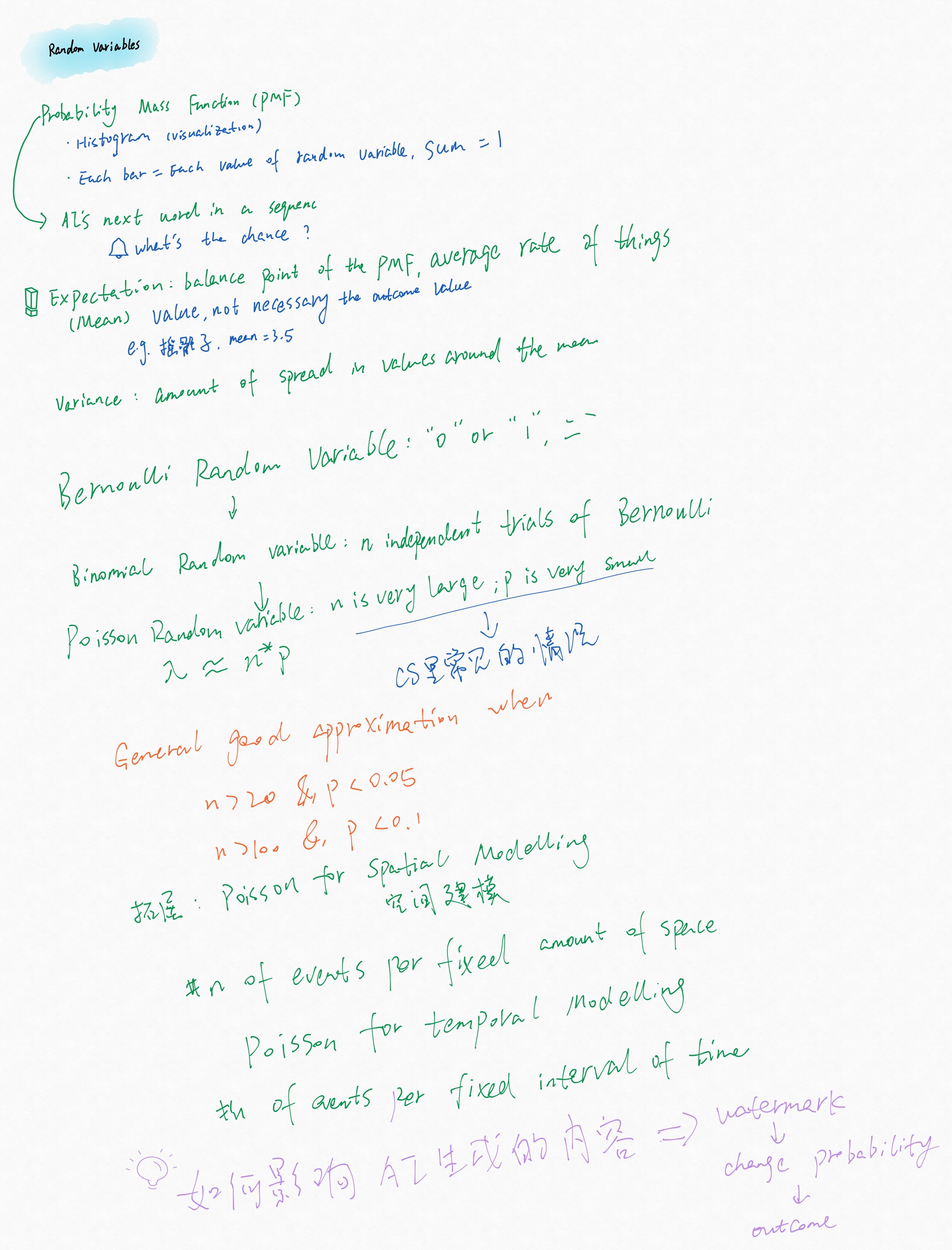
✎ 阅读提示整理后的版本改了这些地方：补上随机变量的定义和骰子例子；“每根柱子 = 随机变量的每个取值”改成柱子对应一个取值、柱高是 P(X = x)，所有柱高之和为 1；期望补上公式 E[X] = Σ x·P(X = x)，“average rate of things”改为长期平均值；方差补上公式 Var(X) = E[(X − μ)²] 和骰子的 2.92；伯努利、二项、泊松补上参数和期望，λ ≈ n·p 写成 λ = np，并说明 n 和 p 的含义；第二条经验法则“n > 100 且 p < 0.1”改为常用的“n ≥ 100 且 np ≤ 10”；“#n of events”改为事件数；水印一行补上具体机制：随机分出绿词并提高它们的概率，再靠数绿词来检测；拼写修正：sequenc → sequence，“not necessary” → “not necessarily”。

✎ 阅读提示What changed in the tidied version: a definition of a random variable with a die example was added; "each bar = each value of random variable" now says each bar is one value and its height is P(X = x), with all heights summing to 1; expectation gained the formula E[X] = Σ x·P(X = x), and "average rate of things" became the long-run average; variance gained Var(X) = E[(X − μ)²] and the die's 2.92; Bernoulli, binomial and Poisson gained their parameters and means, λ ≈ n·p is written λ = np, and n and p are defined; the second rule of thumb "n > 100 & p < 0.1" became the usual "n ≥ 100 and np ≤ 10"; "#n of events" became "number of events"; the watermark line gained the actual mechanism: a random green list whose probabilities are raised, detected by counting green words; spelling: sequenc → sequence, "not necessary" → "not necessarily".

这篇笔记基于我在斯坦福免费在线课程 Probability for AI（PAI，Chris Piech 和 Mehran Sahami 主讲）第二周的学习笔记。定义和例子对照了课程配套读本：

• Chris Piech，Probability for Computer Scientists（CS109 课程读本）中的 PMF、期望、方差、伯努利、二项和泊松分布。
• John Kirchenbauer 等，A Watermark for Large Language Models，ICML 2023（绿词/红词水印与 z 检验）。

动手试一试

• Seeing Theory：Probability Distributions（布朗大学）：拖动参数，看伯努利、二项、泊松等分布的柱状图怎样变化。

This note is based on my study notes from week 2 of Probability for AI (PAI), Stanford's free online course taught by Chris Piech and Mehran Sahami. Definitions and examples were checked against the course's reader:

• Chris Piech, Probability for Computer Scientists, the CS109 course reader: PMF, expectation, variance, and the Bernoulli, binomial and Poisson distributions.
• John Kirchenbauer et al., A Watermark for Large Language Models, ICML 2023 (green/red-list watermarks and the z-test).

Try it yourself

• Seeing Theory: Probability Distributions (Brown University): move the parameters and watch the bar charts of the Bernoulli, binomial, Poisson and other distributions change.