
Stanford · Probability for AI · Week 2, Lesson 1 / PAI002
Random Variables and Three Common Distributions: From the PMF to AI Watermarks
Week 2 of Stanford's Probability for AI (PAI) moves from events to random variables: instead of asking only whether something happens, we give every outcome a number and ask how likely each number is. This note covers the probability mass function (PMF), expectation and variance, and the three distributions computer science uses most: Bernoulli, binomial and Poisson. The last part is the question I found most interesting in class: if we change these probabilities, can we change what an AI writes?
- section
- key term
- reading note
 ELLE · READING COMPANION
Take a moment to connect the ideas
A few foundations, with Elle
Tap a concept to explore it, then try three short questions. You can change any answer.
Random variable and PMF
A random variable X gives every outcome a number, such as the face of a die. Its PMF lists P(X = x) for every value: each bar is one value, its height is a probability, and the heights add up to 1.
Expectation and variance
The expectation E[X] = Σ x · P(X = x) is the balance point of the PMF, the long-run average. The variance E[(X − μ)²] measures how far values spread around it. For a die: 3.5 and about 2.92.
Bernoulli, binomial, Poisson
Bernoulli: one yes/no trial with success probability p. Binomial: successes in n independent Bernoulli trials, mean np. Poisson: events in a fixed time or area, mean λ; with λ = np it approximates a binomial when n is large and p is small.
Watermark
Before each word, the previous word seeds a random split of the vocabulary into green and red words, and green words get a small boost. Detection counts the green words: far more than half means the text is watermarked.
The big picture: from random variables to three distributions
Start with the title at the top, then read the left half: the definition of a random variable, the PMF and its bar chart with a green arrow to "AI's next word", then expectation and variance, each with a die example. The right half runs down the chain Bernoulli → binomial → Poisson; the blue underline marks the condition "n large, p small", the red lines are the rule of thumb for the Poisson approximation, and the green lines extend Poisson to modelling space and time. The purple line along the bottom is the watermark: how changing probabilities steers what an AI generates. My takeaway is in the bottom-right corner.
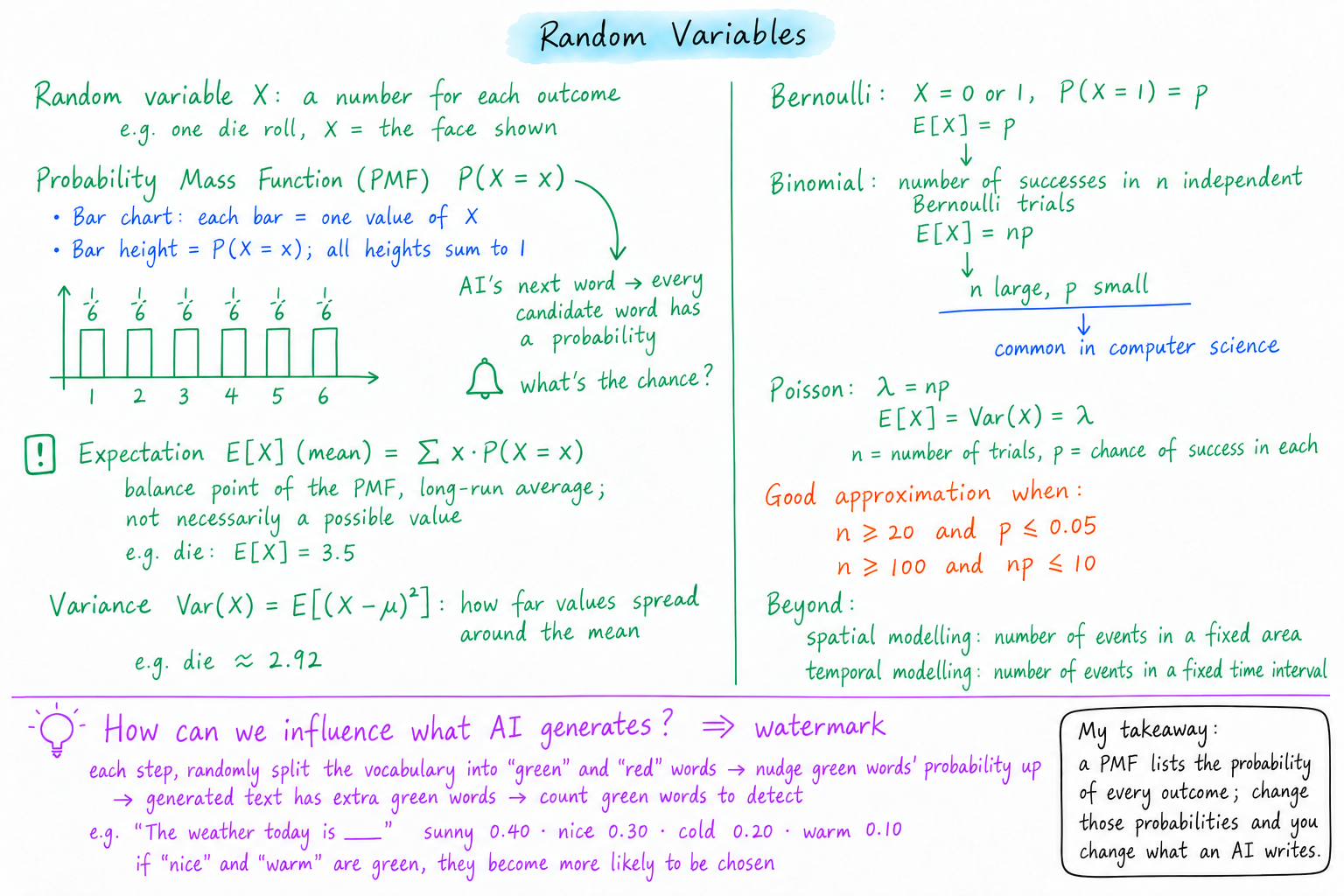
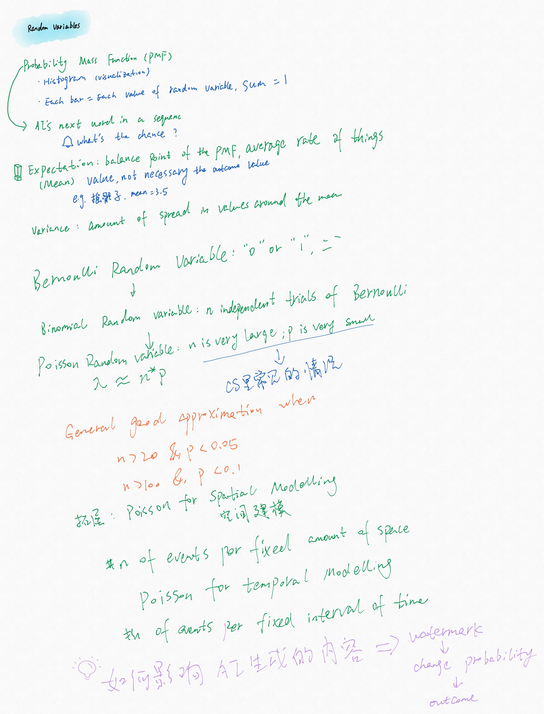
Tidied up from my handwritten page, with a few corrections and additions.
Tap a region to jump to that part of the note; use ⤢ Enlarge to see the full picture.
A random variable gives every outcome a number
A random variable, usually written as a capital X, assigns a number to each outcome of a random experiment. For one die roll, X is the face that comes up, from 1 to 6; for ten coin flips, X can be the number of heads, from 0 to 10.
Once outcomes are numbers we can calculate with them: average them, compare them, measure how spread out they are. Last week's events, such as "roll an even number", can now be written as values of X: P(X ∈ {2, 4, 6}) = 0.5. A lower-case x stands for one particular value that X can take.
The probability mass function: how likely is each value?
The probability mass function (PMF) lists the probability of every possible value of a discrete random variable, written P(X = x). It is usually drawn as a bar chart:
| In the bar chart | Meaning | One fair die |
|---|---|---|
| Each bar on the horizontal axis | One possible value x of X | 1, 2, 3, 4, 5, 6 |
| The height of a bar | P(X = x) | 1/6 for every bar |
| All bar heights together | Must add up to 1 | 6 × 1/6 = 1 |
With data instead of a model, divide the count of each value by the total number of observations: this normalised histogram approximates the PMF.
In AI, every time a large language model generates a word it gives each candidate in its vocabulary a probability. That is a PMF: the bars are words, each height is the chance that the next word is that one, and the heights add up to 1. The model then draws one word from this distribution.
Expectation: the balance point of the PMF
The expectation E[X], also called the mean, multiplies each value by its probability and adds them up:
E[X] = Σ x · P(X = x)
Picture the bars of the PMF as weights resting on the horizontal axis: the expectation is the point where the axis balances. It is also the long-run average if the experiment is repeated many times.
For a die: E[X] = (1 + 2 + 3 + 4 + 5 + 6) × 1/6 = 3.5. No face shows 3.5, so the expectation need not be a value X can take. It tells you where the values average out, not which value is most likely.
Variance: how far values spread around the mean
The variance measures how far the values fall from the mean, written μ = E[X]:
Var(X) = E[(X − μ)²]
The equivalent form Var(X) = E[X²] − (E[X])² is easier to compute. For a die: E[X²] = (1 + 4 + 9 + 16 + 25 + 36) / 6 ≈ 15.17, so Var(X) ≈ 15.17 − 3.5² ≈ 2.92. The square root of the variance is the standard deviation, which has the same units as X and is easier to picture.
Two distributions can share a mean and differ in variance: a die that only ever shows 3 or 4 and one that only shows 1 or 6 both average 3.5, but the second is far more spread out.
Three common distributions: Bernoulli, binomial, Poisson
The three form a chain: a binomial is built from repeated Bernoulli trials, and a Poisson approximates a binomial under particular conditions.
| Distribution | What X counts | Parameters | Mean | Variance | Example |
|---|---|---|---|---|---|
| Bernoulli | 1 if one trial succeeds, otherwise 0 | p: probability of success | p | p(1 − p) | Does one coin flip land heads? Is an email spam? |
| Binomial | Successes in n independent Bernoulli trials | n: number of trials; p: probability of success in each | np | np(1 − p) | Number of heads in 10 coin flips |
| Poisson | Events in a fixed interval of time or region of space | λ: average number of events | λ | λ | Visits to a website in one minute |
Bernoulli has only two outcomes, yes or no. Binomial repeats the same Bernoulli trial n times independently and counts the successes: in 10 flips of a fair coin, the chance of exactly 3 heads is C(10, 3) / 2¹⁰ = 120 / 1024 ≈ 0.117, and on average there are 10 × 0.5 = 5 heads.
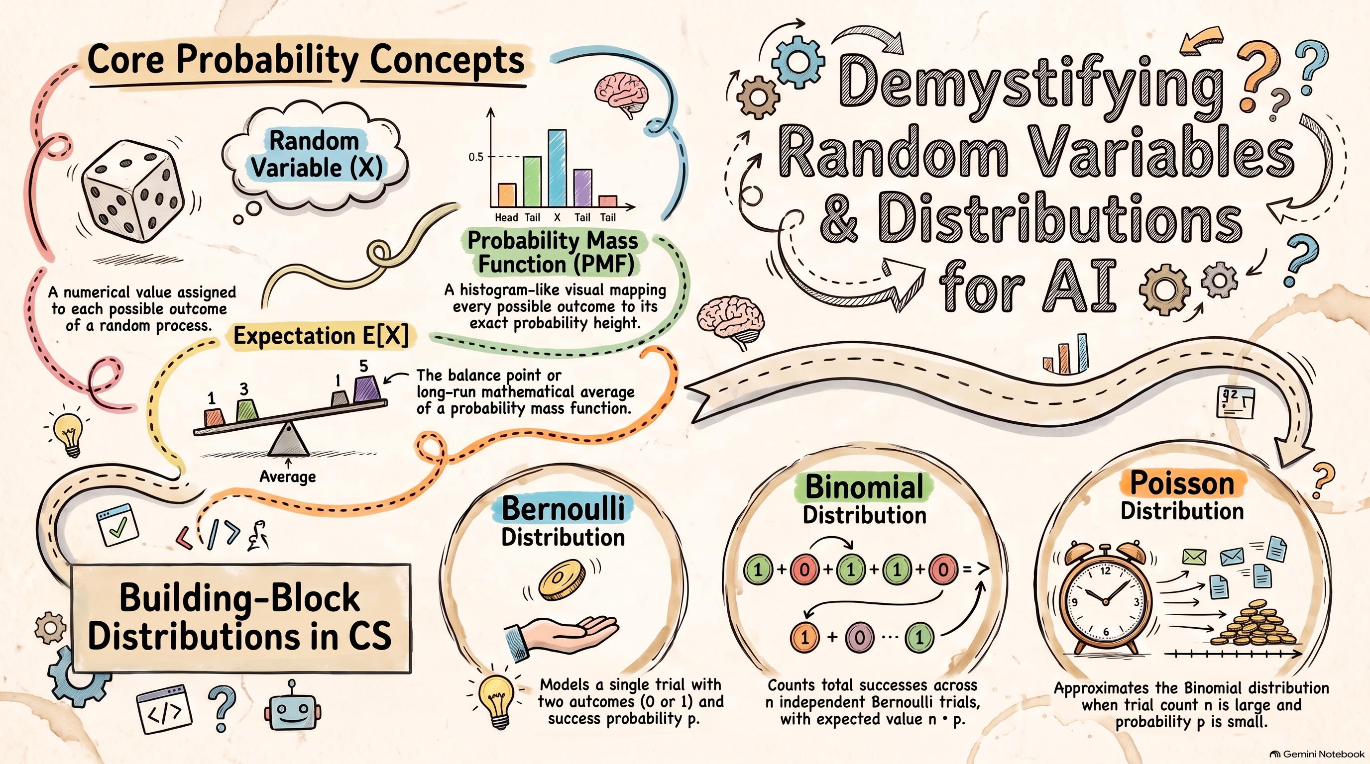
A reading note: the labels under the PMF bar chart (Head, Tail, X, Tail, Tail) do not match any real random variable. Read it as a picture of bars and heights, as in the die table above.
The Poisson distribution: when n is large and p is small
When a binomial has a large number of trials n and a small probability p, computing it directly is awkward, and a Poisson distribution with λ = np approximates it well:
P(X = k) = λᵏ e^(−λ) / k!
An example: a web page gets 1,000 visits a day, and each visit clicks a certain ad with probability 0.002. Strictly, the number of clicks is binomial (n = 1,000, p = 0.002). The Poisson approximation uses λ = 1,000 × 0.002 = 2, so the chance of no clicks at all is e^(−2) ≈ 0.135, almost exactly the binomial answer 0.998¹⁰⁰⁰ ≈ 0.135. The larger n is, the better the approximation.
Common rules of thumb for when the approximation works well:
- n ≥ 20 and p ≤ 0.05;
- n ≥ 100 and np ≤ 10.
"Many trials, each unlikely" is common in computer science: requests reaching a server each minute, typos in a document, packets lost on a network.
Beyond the binomial: modelling space and time. The Poisson distribution is more than an approximation. It counts events in a fixed range directly, as long as they happen independently at a steady average rate.
- Temporal modelling: the number of events in a fixed interval of time, such as patients arriving at an emergency department each hour.
- Spatial modelling: the number of events in a fixed area, such as cases per square kilometre or cells in one microscope field.
A classic piece of history: in 1898 Ladislaus Bortkiewicz counted the soldiers killed by horse kicks each year in corps of the Prussian cavalry and found that these rare events followed a Poisson distribution closely.
Changing probabilities changes what an AI writes: watermarks
Because a large language model samples every word from a PMF over the next word, quietly changing that PMF changes the text it produces. A text watermark does exactly this. In the method of Kirchenbauer and colleagues (2023):
- Split: before each word is generated, the previous word seeds a random split of the whole vocabulary into a "green" list and a "red" list (for example half each).
- Nudge: a constant is added to the score of every green word, so green words become more likely. Red words are not banned.
- Detect: given a text, rebuild each step's green list with the same seed and count the green words. Human writing is about half green; watermarked text has clearly more, and a z-test says how unlikely that is by chance.
An example. The model is completing "The weather today is ___", and the original PMF is: sunny 0.40, nice 0.30, cold 0.20, warm 0.10. If "nice" and "warm" are green at this step, the nudge (δ = 2, a strength used in the paper's experiments) shifts it to about nice 0.62, warm 0.21, sunny 0.11, cold 0.06. All four words can still appear; the choice just leans green. In a 200-word text, a person would write about 100 green words. If we count 150, z = (150 − 100) / √(200 × 0.25) ≈ 7.1, far above the paper's threshold of 4, so the text almost certainly carries the watermark.
Two things to keep in mind: the split is random, not based on how common a word is; and when only one next word makes sense (such as "Barack ___"), the nudge barely changes anything, so text with little room for choice is hard to watermark.
My thoughts
This week has only a few definitions to learn. The probability mass function is shown as a bar chart: each bar is the probability of one possible outcome, and all the bars add up to 1. In AI, it is the chance of each possible next word in a sequence. Expectation and variance are simple to grasp: the expectation is the balance point of the PMF, and the variance is how far the values spread around the mean.
The important part is the three distributions. Bernoulli has only two outcomes, yes or no. Binomial repeats the same yes/no trial many times and counts the successes. Poisson fits the case where n is very large and p is very small; it is used often in practice, and it extends to spatial and time-series modelling.
What interested me most is that changing probabilities can change what an AI generates. Many words could appear in a sentence, but if the probabilities of some of them are raised, the model picks from those words more often, and that is how a watermark is made. One more thing I enjoyed about the course: the instructors talk about the people who discovered these distributions.
Learning sources and resources
This note is based on my study notes from week 2 of Probability for AI (PAI), Stanford's free online course taught by Chris Piech and Mehran Sahami. Definitions and examples were checked against the course's reader:
- Chris Piech, Probability for Computer Scientists, the CS109 course reader: PMF, expectation, variance, and the Bernoulli, binomial and Poisson distributions.
- John Kirchenbauer et al., A Watermark for Large Language Models, ICML 2023 (green/red-list watermarks and the z-test).
Try it yourself
- Seeing Theory: Probability Distributions (Brown University): move the parameters and watch the bar charts of the Bernoulli, binomial, Poisson and other distributions change.