
NLP Learning Notes / NLP006
Neural Language Models: From Word Vectors to Backpropagation
The simple language models in the last note got their probabilities by counting. This note takes a different route: instead of storing a table of counts, a neural network learns what the next word is likely to be. Four concepts carry the idea: neural networks, probability, embeddings and backpropagation. They are also the foundation for what comes next, because large language models (LLMs) are, at heart, very large neural language models.
- section
- key term
- reading note
 ELLE · READING COMPANION
Take a moment to connect the ideas
A few foundations, with Elle
Tap a concept to explore it, then try three short questions. You can change any answer.
Embedding
A word written as a list of numbers so a neural network can compute with it. Words used in similar contexts get similar vectors, and the vectors are learned during training together with the weights.
Weights and bias
Each connection carries a weight. A unit multiplies each input by its weight, adds them up and adds a bias: (0.2 × 10) + (−0.1 × 20) + 0 = 0.
Activation function
A formula applied to the weighted sum that decides what passes to the next layer. ReLU is common in hidden layers, sigmoid gives 0 to 1 for yes/no outputs, and softmax turns the last layer into next-word probabilities.
Backpropagation
After a wrong guess, the error at the output is sent back through every layer to work out how much each weight contributed; then each weight is adjusted. Bigger errors mean bigger changes.
The big picture: from word vectors to backpropagation
Start at the top left. The three green headings are what a language model does (predict a probability distribution for the next word from the words before it), words as vectors, and neural networks. The violet notes define embeddings and list the four key concepts of this note, with a reminder underneath: the weights are the core, and they are learned from data. The blue sketch and its two boxes show how a neuron works: inputs, a weighted sum plus a bias, an activation function, an output; stacked up, these become input, hidden and output layers. The large red box in the middle is the training loop: embeddings pass through the layers to give next-word probabilities, the error is calculated, and the curved arrow carries it back through backpropagation to update every layer's weights. The activation functions are at the bottom left, and my takeaway is at the bottom right.
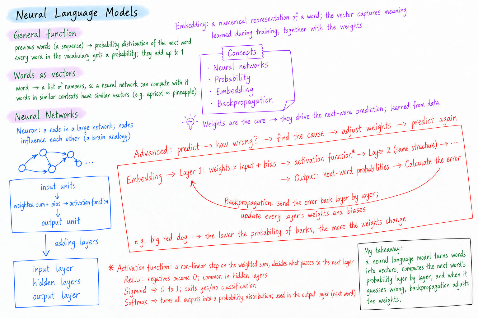
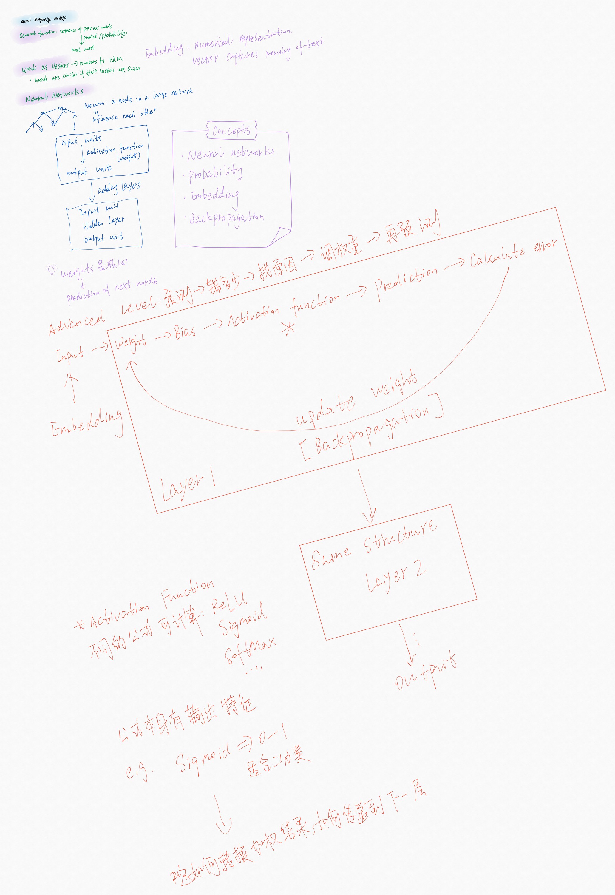
Tidied up from my handwritten page, with a few corrections and additions.
Tap a region to jump to that part of the note; use ⤢ Enlarge to see the full picture.
What every language model computes
However it is built, a language model does one thing: given a sequence of previous words, it computes a probability distribution over the next word. Every word in the vocabulary gets a probability, and together they add up to 1.
| Input: "Next, we list some ___" | Probability of the next word |
|---|---|
| problems | 0.0014 |
| interesting | 0.0043 |
| the, cat | close to 0 |
That one function supports the same two tasks as the count-based models in the last note:
- Generating text: start from a beginning (in LLMs, the prompt), sample a word from the distribution, add it to the sequence, compute the next distribution, and repeat.
- Scoring a sentence: multiply the probability of each word given the words before it to get the probability of the whole sentence.
What changes is where the probabilities come from. A count-based model looks them up in a table of counts; a neural language model computes them with a neural network.
Words as vectors: embeddings
A neural network only handles numbers: a list of numbers (a vector) goes in, and another list comes out. So to build a language model from a neural network, words first have to become vectors. The vectors that represent words are called embeddings.
Representing words as numbers sounds strange, but it has a long history in linguistics. Wittgenstein wrote that the meaning of a word is its use in the language. The course example is tesgüino. After reading "a bottle of tesgüino is on the table," "tesgüino makes you drunk" and "we make tesgüino out of corn," we can guess it is an alcoholic drink like beer. That is the intuition behind distributional semantics: a word's vector should capture the contexts it tends to appear in.
| Method | What each cell counts | What you can compare |
|---|---|---|
| Term-document matrix | How often a word appears in a document, e.g. battle appears 15 times in Henry V | Columns give document similarity; rows give word similarity |
| Word-word co-occurrence matrix | How often a word appears within ±7 words of another, e.g. data appears near information 6 times | Rows: apricot and pineapple have similar vectors, and so do digital and information |
The key result: words that appear in similar contexts have similar vectors. The usual way to measure how alike two vectors are is cosine similarity. Neural language models also represent words as vectors, but in a different way: their embeddings are short, dense vectors that are not counted but learned during training, together with the network's weights.
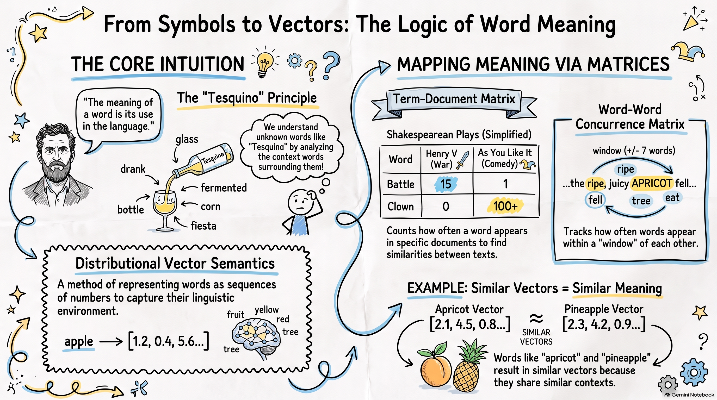
Reading note: the unknown word is tesgüino (the image spells it Tesquino and Tesquina), and "Concurrence Matrix" should be co-occurrence matrix. In the course table, clown appears over 100 times in Twelfth Night, not in As You Like It (6 times), and Henry V is a history play, not a war play.
Neural networks: neurons, weights and layers
The name comes from an analogy: the brain is made of neurons, each a node in a large network, and neurons influence each other through the structure of that network. Artificial neural networks borrow the analogy; they do not simulate a real brain.
The most basic network has input units and an output unit, with a weight on each connection. The output unit first computes the weighted sum of its inputs:
(0.2 × 10) + (−0.1 × 20) = 2 − 2 = 0
A real unit also adds a bias, then passes the result through an activation function:
output = activation(sum of weight × input + bias)
In the course's spam example, the five input units are features of an email: whether the sender is known, whether the title contains win, whether the body contains free, whether there is a personal greeting, and how many words the body has. The weighted sum goes through the activation function and comes out as 0.8, which can be read as an 80% chance that the email is spam.
For harder judgments, you add layers: hidden layers between the input and the output. That sounds complicated, but it is the same basic structure repeated many times; each node is the weighted sum of all the nodes connected to it in the layer before. To make a prediction, the network computes one layer at a time until it reaches the output. This is the forward pass.
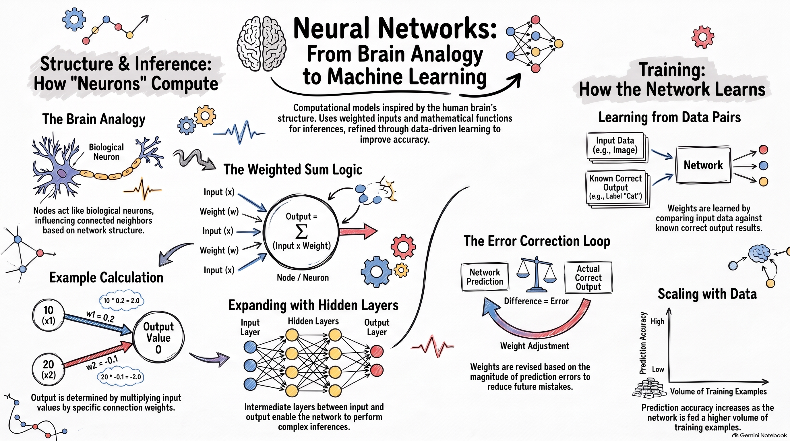
Reading note: the weighted-sum diagram shows only Σ(input × weight). A real unit also adds a bias and applies an activation function; the worked example, whose output is 0, leaves both out, as the course does at first.
Activation functions: what passes to the next layer
An activation function is a mathematical formula applied to the weighted sum. It adds non-linearity: without it, any number of stacked layers would collapse into a single weighted sum. Different formulas have different output ranges, so they suit different places in the network:
| Activation function | What it does | Typical place |
|---|---|---|
| ReLU | Turns negative values into 0 and keeps positive ones: max(z, 0) | Hidden layers |
| tanh | Squeezes values into −1 to 1 | Hidden layers |
| Sigmoid | Squeezes values into 0 to 1 | Binary outputs, such as spam or not |
| Softmax | Turns a whole set of scores into probabilities that add up to 1 | Output layer with many classes, such as which word comes next |
So the activation function decides how the weighted result is transformed and passed on to the next layer. A neural language model ends with softmax: with tens of thousands of words in the vocabulary, it outputs tens of thousands of probabilities, which is exactly the next-word distribution a language model needs. SLP3, Chapter 6
Learning: wrong guesses and backpropagation
Nobody sets the weights by hand; they are learned from data. The training data is a large set of input and correct-output pairs, and the network sees one example at a time:
- Predict: run the forward pass and get an output.
- Calculate the error: compare it with the correct answer.
- Find the cause: backpropagation sends the error back from the output layer through every layer and works out how much each weight and bias contributed to it.
- Adjust the weights: change each one in proportion to its share; bigger errors mean bigger changes (this step is gradient descent).
- Predict again: move on to the next example and repeat.
In the course's travel example, if the correct answer is "didn't like it" and the network outputs 0.001, it is nearly right and the weights barely change. If it outputs 0.89, the error is large and the weights change a lot. The more examples it sees, the lower the error.
One point to keep straight: the error is calculated once, at the output. Backpropagation then passes through all the layers and updates the weights in each one; the layers do not each make and correct their own prediction. SLP3, Chapter 6
Putting it together: a neural language model
Connect these pieces and you have a simple neural language model:
- Input: the previous three words, each replaced by its embedding.
- Hidden layer: weighted sums, a bias and an activation function.
- Output layer: softmax gives every word in the vocabulary its probability of coming next.
Training means predicting the next word, over and over, across a large amount of text. Take "…the big red dog barks against the big pink dog…": the input is big red dog, and the correct next word is barks. The lower the probability the model gives barks, the bigger the error and the more backpropagation changes the weights. Then the window slides one word along, and red dog barks is used to predict against, and so on. Trained this way on text the size of the web, the weights become reliable. The embeddings are learned the same way: they are updated along with the weights.
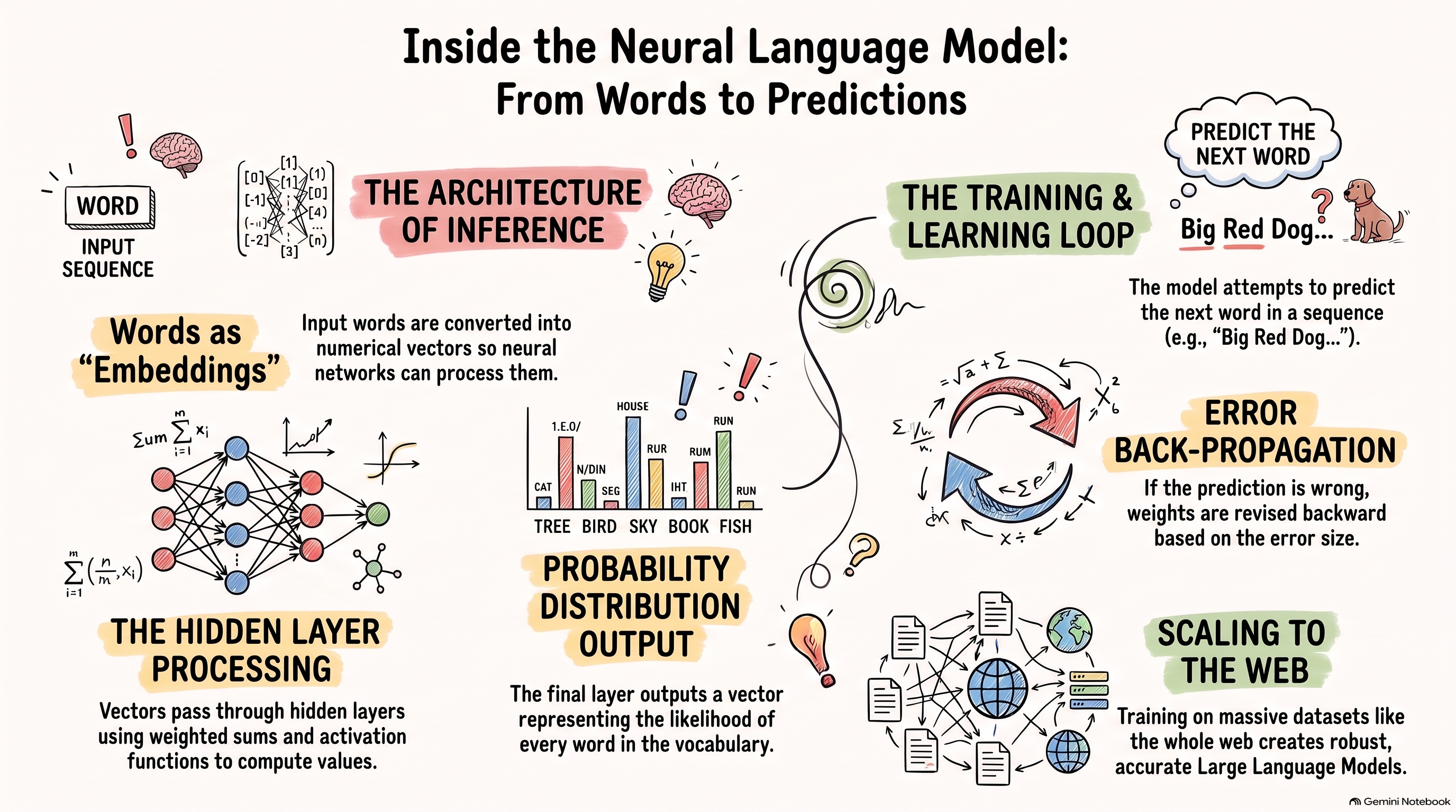
Reading note: the word labels on the bar chart (1.E.O/, N/DIN, SEG and others) are garbled; the chart only stands for one probability per word in the vocabulary.
| Count-based model (last note) | Neural language model | |
|---|---|---|
| Where probabilities come from | Counting and dividing | Computed by a neural network |
| How a word is represented | The word itself, as a symbol | A learned embedding vector |
| An unseen word pair | Probability zero, unless smoothed | Similar words have similar vectors, so it can generalize |
| Generating and scoring | Basic | Better, even with a simple network |
| Cost | Fast, transparent, easy to interpret | Slower to train, uses far more energy, harder to interpret |
What does "generalize" mean here? Suppose training included "make sure that the cat gets fed" but never had gets fed after dog. A count-based model will not predict fed after "the dog gets". A neural language model knows that cat and dog have similar embeddings, so it can predict fed. SLP3, Chapter 6
The large language models in the next note build on exactly this, scaling up both the model and the data.
My thoughts
This note has four concepts to master: what a neural network is; probability, once again; what an embedding is; and what backpropagation is. What a neural language model sets out to do is predict the next word from probabilities, based on the word or words that came before.
To make computation easy for a computer, words have to be turned into vectors. That is what an embedding is: a numerical representation of a word, a vector that captures the meaning of the text. It also means that if two words are similar, their vectors are similar too.
Neural networks borrow the analogy of the brain's neural networks. A neuron is a point in the network, and neurons influence each other; you can think of it as neurons possibly being related. To build the network, you start with input units, then go through an activation function (a mathematical formula; different purposes call for different formulas) to reach the next output unit. This step can repeat over many layers until you get the final result. So in this network, the weight on each neuron's connections affects the prediction of the next word.
While the model is being built, it keeps correcting itself: predict first, see how wrong it is, find the cause, adjust the weights, and predict again. That is where backpropagation comes in.
Learning sources and resources
This note is based on my study notes from the University of British Columbia (UBC) micro-certificate program "Natural Language Processing to Improve Patient Care," in the course "Overview of NLP and Large Language Models" (the Neural Language Models lecture by Giuseppe Carenini). Technical details were checked against Jurafsky and Martin, Speech and Language Processing (3rd edition draft, August 2026): Chapter 5, Embeddings and Chapter 6, Neural Networks.
Try it yourself
- TensorFlow Playground: build a small neural network in your browser, add or remove hidden layers, switch between ReLU, tanh and sigmoid, and watch the error fall during training.
- GeeksforGeeks: Activation Functions in Neural Networks: the three above are only examples; this page lists many more (linear, tanh, Leaky ReLU, ELU and others), each with its formula and a graph.
- Embedding Projector: explore real word vectors in 3D; search for a word and see which words sit closest to it.